 Ofir Steinherz

We have a database we know inside out. It’s consistent and readable. We have another database, but we can’t exactly call it consistent; its main column is entered manually. The task: analyze both databases together. Sound familiar?
It certainly does to me; I’ve been there. As part of my military service, I compared a standardized database with one written by hand. How did I do it, you ask? With dozens of hours of manual work. The main drawbacks of working this way:
Valuable working time that we’d rather spend on other things. What’s more, all that work can lead to burnout, which we certainly want to avoid.
The time spent working leads to a greater margin of error, potentially making the information even less reliable than it already is.
Repeatability isn’t possible, and we have to classify everything all over again each time. No fun at all.
After reading this article, you’ll know how we can automate this process, step by step:
- First Steps 👣
- Getting to Know the Databases 🔎
- Matching Columns 🔗
- Analyzing the Findings 🤔
- This Is Just the Beginning 😎
#First Steps 👣
#Libraries
Before I begin, I used Jupyter as my IDE, running locally.
import pandas as pd
pd.set_option('display.float_format', lambda x: '%.3f' % x)

import numpy as np

from fuzzywuzzy import process

import matplotlib.pyplot as plt
import seaborn as snspandas(lines 1–2) - We’ll use it for data analysis inPython. On the second line, I configured it so I could see very large and very small numbers without the development environment rounding them.numpy(line 4) - A library that serves as a foundation for the vast majority of libraries in the field. EvenPandasis built on it.fuzzywuzzy(line 6) - The library we’ll use to compare the columns.matplotlibandseaborn(lines 8–9) - Libraries for creating charts.
#Where the Databases Came From
This article is based on the government data repository Data Gov. As someone who loves data, I think this site really is every Data Analyst’s dream. You can find data on a variety of topics: Israel’s economy, transportation, health, and more.
I decided to investigate whether there is a relationship between the number of bank branches and the number of residents in Israeli cities.
#Getting to Know the Databases 🔎
I downloaded the databases to my computer manually, then loaded the CSV files using Python. Data Gov actually supports API, but in this case I decided to keep things simple.
#Banks
I had no trouble accessing the bank database. In the following code snippet, I imported the local CSV file and printed the column names.
snifim = pd.read_csv('snifim_he.csv')

snifim.columns
👇🏼
Index(['Bank_Code', 'Bank_Name', 'Branch_Code', 'Branch_Name',
       'Branch_Address', 'City', 'Zip_Code', 'POB', 'Telephone', 'Fax',
       'Free_Tel', 'Handicap_Access', 'day_closed', 'Branch_Type', 'Open_Date',
       'Close_Date', 'Merge_Bank', 'Merge_Branch', 'X_Coordinate',
       'Y_Coordinate', 'ban_city', 'final_city'],
dtype='object')
In this database, we’ll mainly use the Bank_Name and City columns.
#Population
If we take a look at the CSV containing the population figures for each locality, we can see that the text is unreadable and the columns aren’t laid out properly. We have a problem.
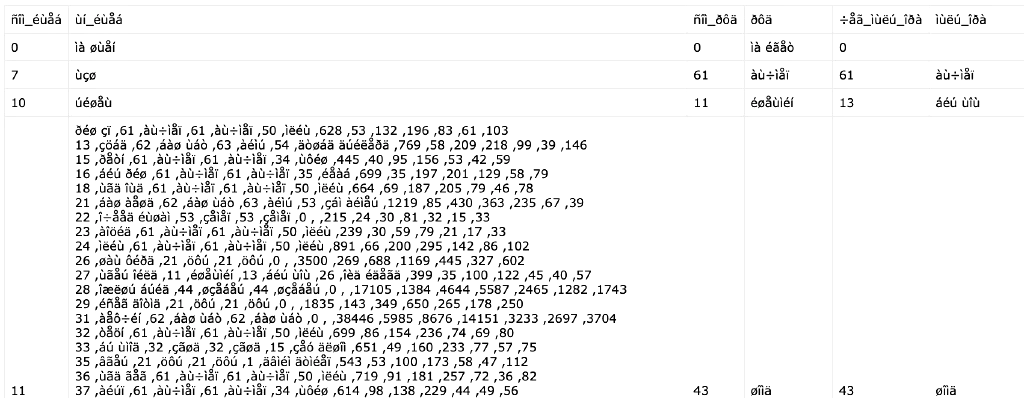
I concluded that both the computer and IDE need to be told explicitly which encoding to use when reading the file. After some research, I determined that the relevant encoding was ISO-8859-8.
population = pd.read_csv('residents_in_israel_by_communities_and_age_groups.csv',encoding='ISO-8859-8')
population = population.applymap(lambda x: x.strip() if isinstance(x, str) else x)

population.columns
👇🏼
Index(['סמל_ישוב', 'שם_ישוב', 'סמל_נפה', 'נפה', 'קוד_לשכת_מנא', 'לשכת_מנא',
       'קוד_מועצה_אזורית', 'מועצה_אזורית', 'סהכ', 'גיל_0_5', 'גיל_6_18',
       'גיל_19_45', 'גיל_46_55', 'גיל_56_64', 'גיל_65_פלוס'],
dtype='object')
Reading
population(line 1) - We’ll use the same function we used to read the bank branch database, but this time we’ll set theencodingparameter to theISO-8859-8encoding.Editing
population(line 2) - We’ll remove unnecessary spaces using thestripfunction.
In this database, we’ll mainly use the שם_ישוב' and סהכ columns.
#Initial Exploration 🧠
#Banks
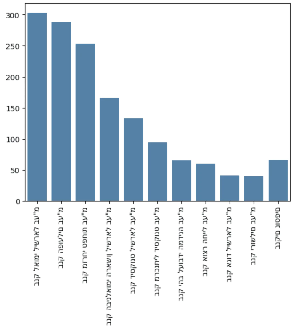
Besides running snifim.head(), I thought it would be nice to show the 10 largest banking companies in Israel.
First, I wrote a relatively simple function that sorts the df and returns the num_of_rows by size.
def shorten_df(df, iterate_row, num_of_rows, comment):
    sum_df = df[iterate_row].value_counts(ascending=True)
    length = len(sum_df)

    top_rows = sum_df[num_of_rows:].sort_values(ascending = False)

    if num_of_rows < length:
        other_rows = sum_df[:length - num_of_rows]
        remaining_row = pd.Series(other_rows.sum(), index=[comment])

        rows_plot = pd.concat([top_rows, remaining_row])
        return rows_plot
    return sum_df
Then I could easily see the 10 largest banking companies in Israel and display a chart:
banks = shorten_df(snifim, 'Bank_Name', 10, 'בנקים נוספים')

ax = sns.barplot(x = banks.index, y = banks.values)
ax.set_xticklabels(ax.get_xticklabels(),rotation = 90)

plt.show()
Although we managed to show the branches in a chart as I wanted, I ran into a problem displaying Hebrew that I still haven’t been able to solve. If anyone knows a solution, I’d love to hear it 😧.
Before moving on to the population database, I decided to check how many unique cities there are in this database:
ban_cities = set(snifim['City'])
print("Banks unique cities: {0}".format(len(ban_cities)))
👇🏼
"Banks unique cities: 161"#Population
For the population data, I decided to run a basic groupby to get a sense of the scale and see whether the data made sense:
population.groupby('שם_ישוב')['סהכ'].sum().sort_values()
👇🏼
כפר עבודה              1
ידידה                  2
כרי דשא                3
איתנים                 4
אורנים                 5
                  ...
ראשון לציון       277915
פתח תקווה         278645
חיפה              331402
תל אביב - יפו     573660
ירושלים          1056097
Name: סהכ, Length: 1264, dtype: int64
Here, too, I checked how many unique cities there are in the database. Notice the difference!
pop_cities = set(population['שם_ישוב'])
print("Population unique cities: {0}".format(len(pop_cities)))
👇🏼
"Population unique cities: 1264"#Matching Columns 🔗
#What’s the Problem?
Both databases have a column referring to the city. The problem is that the city names aren’t written the same way. For example, we can see that “Nahariya” is written with two instances of the Hebrew letter yod in the bank database, but with just one in the population database 🤬.
'נהרייה' in ban_cities 👉🏼 True
'נהריה' in pop_cities 👉🏼 True#The Levenshtein Distance Algorithm
I first encountered this algorithm while studying the Data Scientist with Python track on Datacamp. In addition to my explanation, I highly recommend learning about the mathematical background in this Medium article.
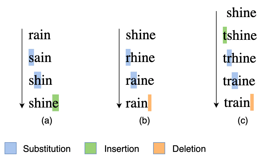
Given two str, we get a number representing the distance between them. What do I mean by distance? The number of the following operations we need to perform to get from one str to the other:
- Inserting a character 🧩
- Deleting a character ⌫
- Replacing a character 🔄
#So How Do We Calculate the Distance?
Using the process function, which we imported along with the fuzzywuzzy library, we can calculate the distance between words. In this example (copied from Datacamp), we want to find the element in the strOptions array that is closest to str2Match:
str2Match = "apple inc"
strOptions = ("Apple Inc.", "apple park", "apple incorporated", "iphone")
Ratios = process.extract(str2Match,strOptions)
print(Ratios)
👇🏼
[('Apple Inc.', 100), ('apple incorporated', 90), ('apple park', 67), ('iphone', 30)]
We got an array neatly containing the values from the strOptions array and their relative distance from str2Match. That’s it! Now we can return to our task and compare the cities in the databases 🥳.
#Calculating the Distance Between City Names
Now for the most fun part: applying the distance algorithm to the databases. I decided to match the bank database against the population database based on intuition and the difference in the number of cities.
ban_and_pop_city = pd.DataFrame(columns=['ban_city', 'pop_city', 'ratio'])

for ban_city in ban_cities:
    Ratios = process.extract(ban_city,pop_cities)[0]

    city_row = {
        'ban_city': ban_city,
        'pop_city': Ratios[0],
        'ratio': Ratios[1]
    }
    city_row = pd.DataFrame(city_row, index=[0])

ban_and_pop_city = pd.concat([ban_and_pop_city, city_row], ignore_index = True)ban_and_pop_city(line 1) - Creating an emptydfwhere we’ll put the city names from the bank database and their corresponding cities in the population database.for ban_city(line 3) - A loop that goes through the city names in the bank database.process.extract(line 4) - Finding the city name in the population database that is closest toban_city.city_row(lines 6–11) - Creating a new row for a city that we can insert into theban_and_pop_cityfrom earlier.pd.concat(line 13) - Insertingcity_rowintoban_and_pop_city.
#How Are the Match Percentages Distributed?
It was important to me to get an overview of how the matches were distributed, especially where they were concentrated.
sns.histplot(data=ban_and_pop_city, x="ratio", bins=20)
plt.show()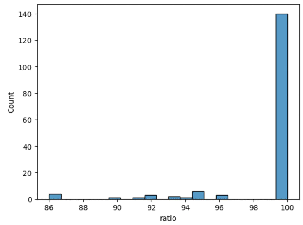
We’re in good shape: most cities have a 100 percent match. But our next task is to figure out which cities don’t.
#So Which Cities Have Low Match Scores?
At a glance, we can see that most discrepancies stem from cases like the example at the beginning: cities spelled with either one or two instances of yod. Let’s investigate which city names didn’t contain two instances of yod and weren’t a perfect match:
without_youd = ban_and_pop_city[ban_and_pop_city['ratio'] < 100]
without_youd = without_youd[~without_youd['ban_city'].str.contains('יי')]| index | ban_city | pop_city | ratio |
|---|---|---|---|
| 73 | Airport City | Kiryat Ye’arim (institution) | 86 |
| 109 | Ben-Gurion Airport | Kerem Ben Zimra | 86 |
| 131 | Tel Aviv -Yafo | Tel Aviv - Yafo | 96 |
| 139 | Arava Regional Council 54 | Kaukab Abu al-Hija | 86 |
| 140 | Northern Negev Highlands Regional Council 48 | Har Gilo | 86 |
| 153 | Ramla Area (not assigned to a locality) | Ramla | 90 |
#Manual Changes
As we can see in the table above, there are edge cases we’ll need to edit manually. We haven’t eliminated manual work entirely; instead, we’ve moved from a manual workflow to a bird’s-eye review, saving most of the working hours in the process.
city_df = ban_and_pop_city
city_df['final_city'] = city_df['pop_city']

city_df.loc[city_df['ban_city'] == 'נמל תעופה בן-גוריון', 'final_city'] = 'לוד'

city_df[city_df['pop_city'].str.contains('נמל תעופה בן-גוריון')]city_df(lines 1–2) - We created a copy ofban_and_pop_cityto serve as our dictionary. Thefinal_citycolumn will contain the final city names.city_df.loc(line 4) - We’ll manually filter the city names we want to change. For example, we’ll classify a bank at the airport that was initially assigned to Kerem Ben Zimra as being in Lod.contains(line 6) - We’ll check the changes we made.
#Merging the Tables 😲
Now that we have a dictionary (city_df), we can use it to convert the city names in the snifim table so we can join it to the population table:
#In the population Table
population = population.merge(
  city_df[['pop_city','final_city']],
  left_on='שם_ישוב',
  right_on='pop_city',
  how='left'
)#In the snifim Table
snifim = snifim.merge(
  city_df[['ban_city', 'final_city']],
  left_on = 'City',
  right_on = 'ban_city',
  how = 'left'
)#Analyzing the Findings 🤔
#Which Cities Have No Banks?
First of all, I decided to find out what percentage of cities have at least one bank:
population['has_bank'] = np.where(population['final_city'].isnull(), False, True)
length = len(population['final_city'])
no_banks = (population['has_bank'] == False).sum()

print("Percentage of cities with banks: {0:.0%}".format((length - no_banks) / length))
👇🏼
"Percentage of cities with banks: 13%"has_bank(line 1) - If the merge operation returnednull, we can infer that there is no bank in that city. The value in this column is Boolean.length(line 2) - Represents the number of cities we have in the population table.no_banks(line 3) - Adds up the number of cities with no banks.
87% of Israeli localities don’t have even a single bank branch. Surprising, right? Let’s show that in a chart:
pop_no_banks = population[population['has_bank'] == False]

sns.histplot(data=pop_no_banks, x="סהכ")
plt.axvline(x=pop_no_banks['סהכ'].median(), color='red')

plt.show()pop_no_banks(line 1) - For simplicity, I added adfto hold the details of cities with no bank branches.sns.histplot(line 3) - I plotted the distribution of population sizes by the number of localities.plt.axvline(line 4) - I displayed the median on the chart.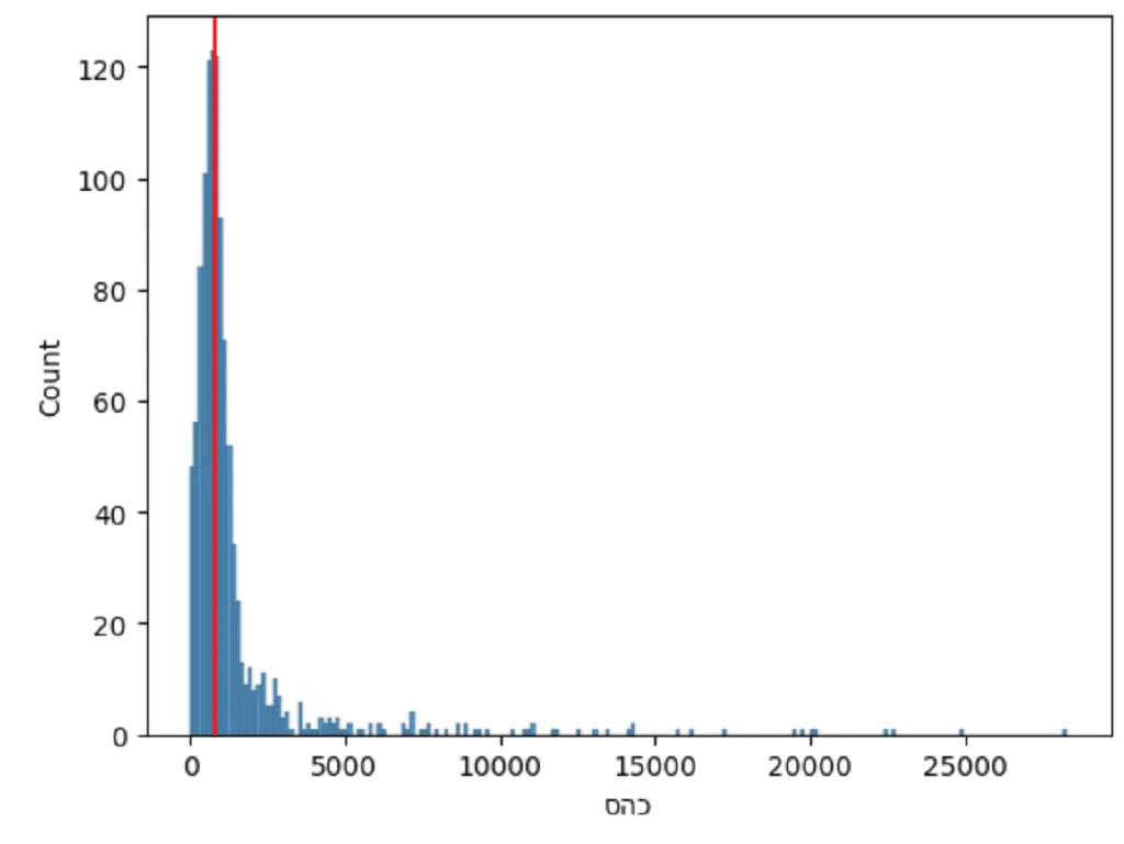
#Distribution of Medium-to-Large Cities Without a Branch
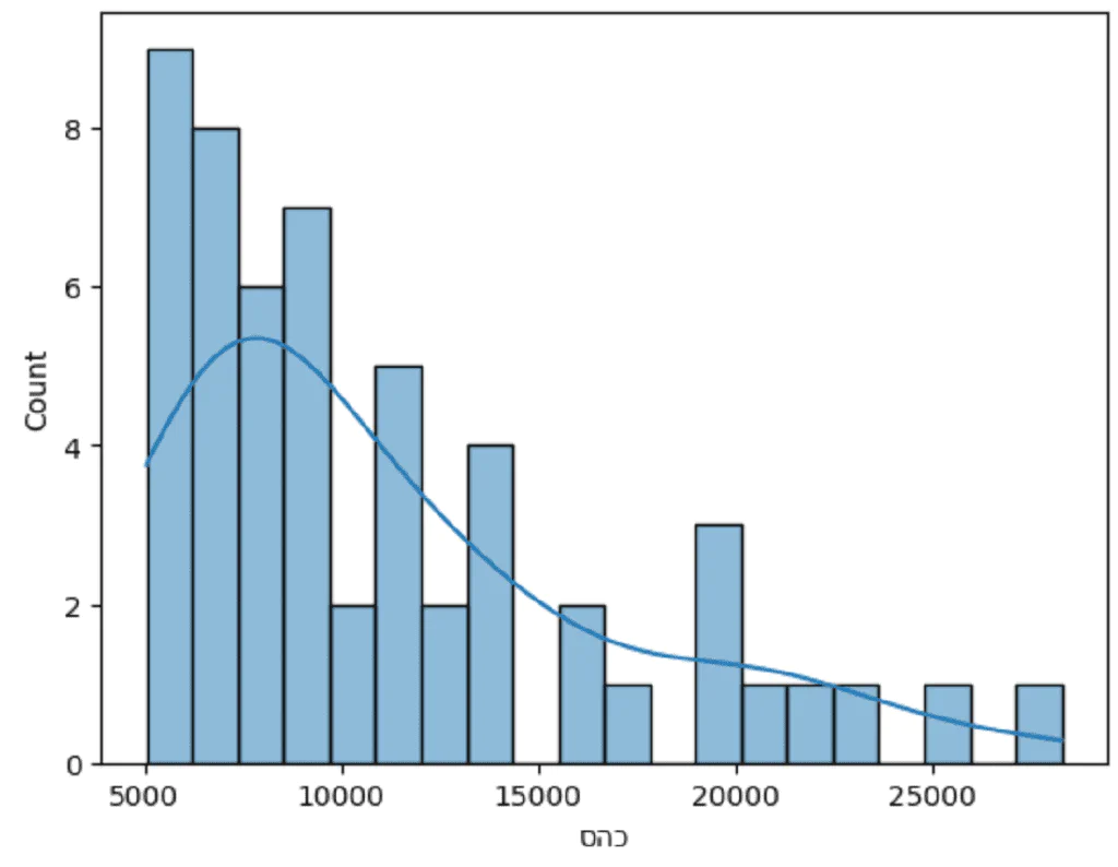
As we can see from the chart above, it makes a lot of sense that localities with up to 5,000 residents wouldn’t have bank branches. I decided to examine the distribution of cities with no bank branches and more than 5,000 residents.
sns.histplot(
    data=pop_no_banks[pop_no_banks['סהכ'] > 5000],
    x="סהכ",
    bins = 20,
    kde = True
)
#Distribution of the City Groups
The next step that interested me was comparing the distributions of cities with no bank branches against those with branches.
plt.xlim(0, 1000)
ax = sns.histplot(population, x="סהכ", hue="has_bank")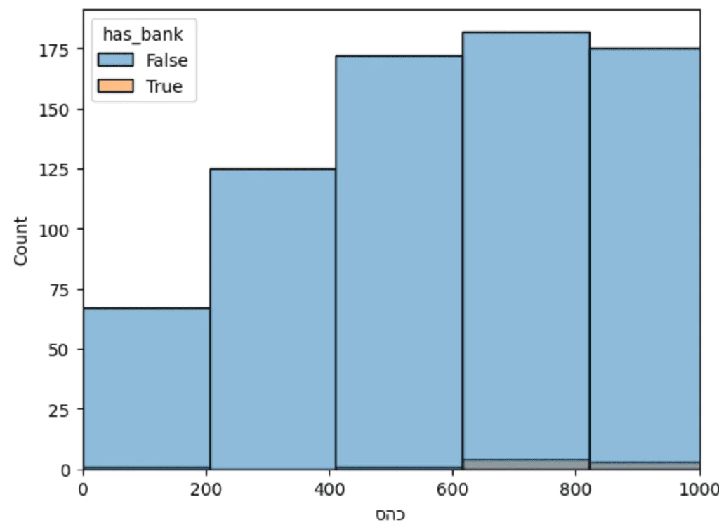
We made a simple histogram, just like in the previous section, but ran into a problem: the groups are on different scales.
#The Data Binning Process
#What Is It, Anyway?
To compare and examine the distributions of the groups, we’ll need to divide them up evenly. To do this, we’ll use a process called Binning. This process divides the values into equal ranges and assigns each value to the appropriate range. We’ll consider this a Data Preprocessing step.
#Dividing Up the Values
pop_bind = population.copy()
min_val = 2500
max_val = 75000
num_bins = 30

bins = np.linspace(
    min_val,
    max_val,
    num_bins
)

pop_bind['b_pop_y'] = pd.cut(pop_bind[pop_bind['has_bank']]['סהכ'], bins=bins, include_lowest=True, precision=0)
pop_bind['b_pop_n'] = pd.cut(pop_bind[~pop_bind['has_bank']]['סהכ'], bins=bins, include_lowest=True, precision=0)pop_bind(line 1) - I created a copy ofpopulationto avoid “messing it up” and keep the data clean.- Range variables (lines 2–3) - Variables that help us decide the range of total population sizes per city that we want to divide up.
num_bins(line 4) - Stores the number of bins we want to divide the data into.np.linspace(lines 6–10) - A function fromNumpythat takes a range of values and the number of bins we want to divide it into. The function returns abinsarray containing the upper value of each range. For example: 2,500, followed by 5,000, and so on.pd.cut(lines 12–13) - A function fromPandasthat divides values according tobins:- For each row in the table, the function takes the value (
סהכ) and checks which range inbinsit belongs to. For example, the city in row 1,261, with 33,299 residents, was assigned to the range (32500.0, 35000.0]. pandas._libs.interval.Interval- The type of value we get from thecutfunction. It tells us which range theסהכbelongs to.- I ran the function separately for cities with banks and cities without, so I could compare them later.
- For each row in the table, the function takes the value (
#Combining the Columns
To compare the distributions, the next step is to combine the b_pop_y column with the b_pop_n column.
pop_bind['b_pop'] = pop_bind['b_pop_y'].fillna(pop_bind['b_pop_n'])#Preparing the Visualization
The next step was to prepare a summary table, to_plot, that counts how many cities there are in each group.
to_plot = pop_bind.groupby(['b_pop','has_bank'])['סהכ'].count().reset_index()| b_pop | has_bank | Total | |
|---|---|---|---|
| 0 | (2499.0, 5000.0] | False | 57 |
| 1 | (2499.0, 5000.0] | True | 6 |
| 2 | (5000.0, 7500.0] | False | 18 |
| 3 | (5000.0, 7500.0] | True | 8 |
| 4 | (7500.0, 10000.0] | False | 12 |
| 5 | (7500.0, 10000.0] | True | 10 |
#Visualization
Now, using a relatively simple barplot function, we can visually compare the concentration of cities with bank branches against those without.
sns.barplot(x = 'b_pop',
            y = 'סהכ',
            data = to_plot,
            hue = 'has_bank')
plt.xticks(rotation=90)

plt.show()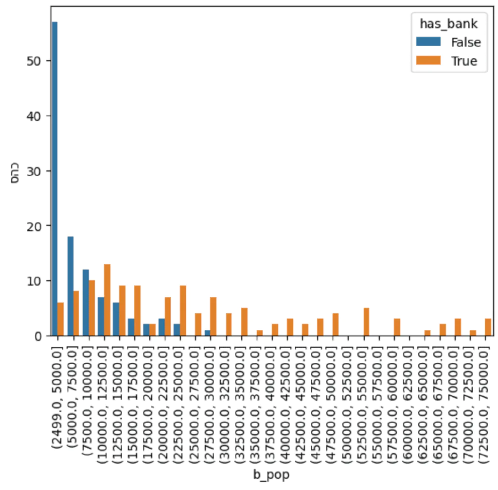
#The Relationship Between the Total Number of Bank Branches and Population
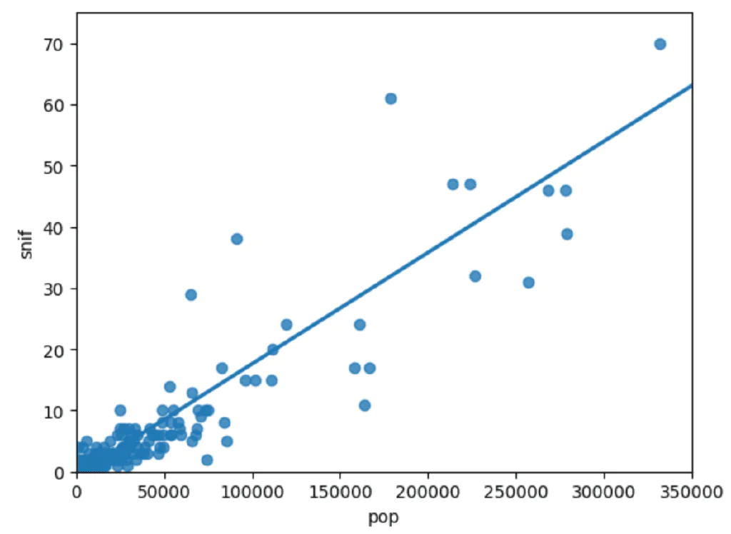
I was curious to check whether there is a relationship between the total number of bank branches and the number of residents in each locality.
snif = snifim.value_counts('final_city')
pop = population.groupby('שם_ישוב')['סהכ'].sum()

snif_pop = pd.concat([snif, pop], axis=1)
snif_pop.columns = ['snif', 'pop']
snif_pop = snif_pop[~snif_pop['snif'].isna()]snif(line 1) - How many branches there are in each city.pop(line 2) - How many residents there are in each locality.snif_pop(lines 4–5) - A merged table.isna(line 6) - I removed cities with no banks.
plt.xlim(0, 350000)
plt.ylim(0, 75)

sns.regplot(x="pop",
            y="snif",
            data=snif_pop,
            ci=None)

plt.show()lim(lines 1–2) - Setting the ranges for the x-axis and y-axis. I excluded the outlier cities, Tel Aviv and Jerusalem.sns.regplot(lines 4–7) - Creating a scatterplot with a linear trend line showing the relationship.
#This Is Just the Beginning 😎
Now that we’ve learned about several distinctive technologies, we can take our research even further, expanding the dataset and presenting it in ways we hadn’t considered before.
The most important thing I want to leave you with is to remember, throughout the research, what message we want to convey and what we’re actually investigating. Otherwise, we’ll lose our way and won’t have a clear bottom line.