Word2Vec for Beginners 📒

Many people are familiar with ChatGPT and use it every day. The tool has become synonymous with artificial intelligence technologies, and it is undoubtedly revolutionizing the way we consume and create content. This shift in perspective sparked my interest in the field of language. In this post, we will learn the basics of natural language processing (NLP), explore language models in the field of Word to Vector (Word2Vec for short), and see how we can use them to represent the semantic meaning of words.
Vectors #
What are they? Why are they important? Vectors are collections of numbers that together represent meaning. A vector is represented in a space, so every time we add a feature to a vector, we also add a new dimension. In our case, each vector represents a word, so if two vectors are close together, we can infer that the words have similar meanings. The process of embedding words as vectors is called word embeddings.
As an analogy, let’s consider the world of royalty. If we “remove” masculinity from a king and add femininity, we can infer that we will get a queen. What we actually did was perform a mathematical operation on words. That mathematical operation produced the most fitting result we could imagine. Let’s dive a little deeper and see how this works in practice.
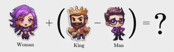
What Does a Vector Look Like? How Can We Use Vectors? #
The first step we need to take is to build vectors that represent the meaning of each word. In our case, we want to distinguish between king, queen, man, and woman, and we will choose three main features for our feature vectors: royalty, gender, and power. A king and queen belong to a kingdom, so they received 1.0 for both royalty and power. For gender, a man gets a value of minus one and a woman plus one (without implying, of course, that men are inferior to women).
| Power | Gender | Royalty | Vectors |
|---|---|---|---|
| 1.0 | -1.0 | 1.0 | King |
| 0.5 | -1.0 | 0.0 | Man |
| 0.5 | 1.0 | 0.0 | Woman |
| 1.0 | 1.0 | 1.0 | Queen |
Each feature of the vector represents a new dimension, so each of the four vectors we built has three dimensions. By combining these three dimensions, we have obtained a representation of the meaning of each word.
The second step is to calculate the result of the mathematical operation, which we will represent using the vector names: “King - Man + Woman”. We take the vector representing the word “King”, subtract the vector for “Man”, and add the vector for “Woman”. The result is a new vector in the space. We check which word is closest to the resulting vector and find that “Queen” is the closest. Through this simple example, we can see that the model has learned relationships between words.
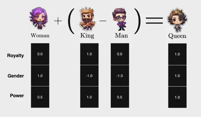
Our result matches the vector representation of the queen in the hypothetical world we created. Note that this example is simplistic; if we had to characterize every single word in the language, there would be thousands of features, accuracy would be low, and the task would be very difficult. That is why, in Word2Vec models, the feature vector values are determined using machine learning, so that the vectors span a space of hundreds of dimensions, and their values cannot be directly interpreted by humans.
To avoid having to manually go through every single word and decide on its feature vector values, we will use a neural network, training it so that, for every two consecutive words, it calculates the probability that the next word will be each of the words in our vocabulary. As a byproduct of this process, we will get a word embedding, since for each pair of words we will get a ranked list of probabilities that a particular word comes next. Words with high, similar probabilities are likely to have similar meanings along certain dimensions, even if their meanings are not identical. We will soon dive into an example that will help make this clearer.
The Problem #
The problem we want to solve is word completion. During training, we will use many texts as part of the dataset. For the sake of explanation, I wrote a sample paragraph:
Let’s take a sentence. For example, given the context “ordered his ministers ____”, we will find the most suitable word, the target word. From experience, we know that the word intelligence does not fit, nor do the or time. However, the word Emperor does fit the context, as does King. This lets us infer that these two words have similar meanings.
Emperor ordered his ministers
Now that we have found a problem we want to solve, we need to build the dataset on which we will train the neural network using CBOW (short for Continuous Bag of Words). The dataset will consist of two parts, context and target word:
ordered, his -> King
gather, intelligence -> to
Neural Networks #
Background #
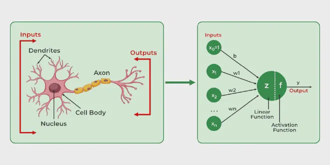
Before we start training a neural network on our dataset, let’s go over some background together. A neuron (sometimes called a node) is the most basic building block of an artificial neural network. The structure of a neuron is inspired by the biological structure of the human brain. In practice, a neuron receives input, performs mathematical calculations on it, and returns the result as output.
When many neurons are connected, they form a neural network, which can make more complex decisions than a single neuron. The network’s goal is to understand the relationship between input and output. The network learns from a variety of examples and adjusts itself so that it can make predictions based on information it has not seen before.
A Neuron #
Components of a Neuron #
Input - Each neuron has a defined number of inputs. This is the gateway into the neuron, a sort of connecting pipeline. The input can be raw external data or the result of a calculation by another neuron in the network.
Weights - Each input has a corresponding weight, which determines its importance in determining the result. Initially, the weights are set randomly, and during learning their values are adjusted to achieve better predictions. After training, the weight values become fixed.
Bias - An additional parameter in the neuron that allows flexibility and shifting. This value is added to the sum of the weights.
The Calculation Process #
- Summation Function (Linear Combiner) - For each input, the neuron multiplies its value by the corresponding weight and sums the products for all inputs (weighted sum). We can see that if a weight is close to zero, its associated input will have little effect on the accumulated sum, and vice versa.
- Adding Bias - After summing the products, we add a bias to the function. The bias lets us adjust the neuron’s output independently of the input values.
- Activation Function - Adding the bias to the sum of the products gives us a value that we feed into an activation function. The function’s purpose is to calculate a nonlinear relationship between the neuron’s input and output. There are various types of activation functions, and we will focus on the familiar sigmoid function. This function transforms the sum of the inputs into a value between 0 and 1.
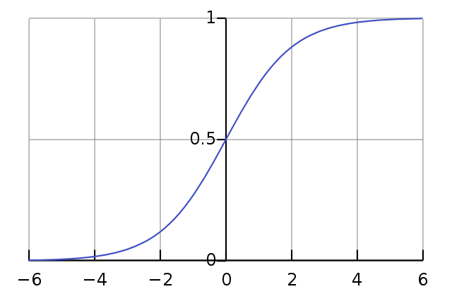
To sum up, each neuron receives a collection of inputs, multiplies them by the weights determined during training, adds a bias, and feeds the result into an activation function. It passes the result to the next neuron or returns it to the user as output.

A Neural Network #
Components of a Neural Network #
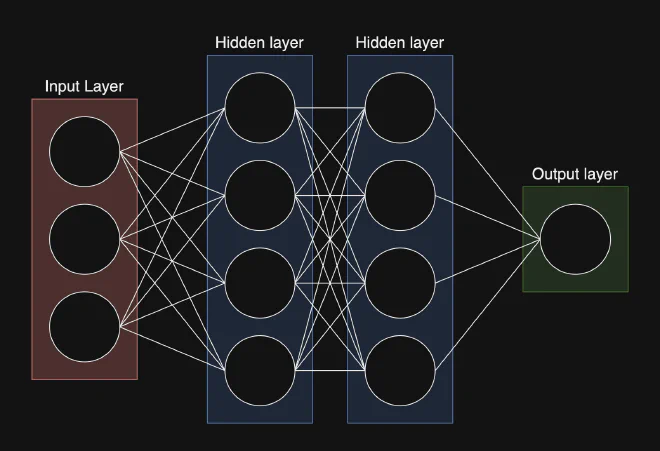
A neural network consists of a collection of neurons arranged in several layers, with a defined number of neurons in each layer. In practice, the network performs fairly simple mathematical operations, and its main intelligence lies in its weights and structure.
- Input Layer - This is where the information we want to process through the neural network enters. It receives raw input and then passes it to the subsequent layers. The number of neurons in the layer corresponds to the number of features in the dataset.
- Hidden Layers - The hidden layers perform calculations based on the input. Every neuron in these layers contributes to the network’s final answer. We can have as many hidden layers as we want, and define the number of neurons in each one.
- Output Layer - Based on the input and the network’s processing, this layer returns the output of the calculations. The number of neurons in this layer corresponds to the number of possible outputs.
Operations #
Every neural network follows a sequence of operations through which its weights are adjusted to the dataset:
- Forward pass - The neural network receives input, processes it according to the weights of its constituent neurons, and returns output. This output is essentially the neural network’s prediction.
- Loss Function - The amount of error: the difference between the prediction and the correct value.
- Backward pass - Sometimes also called backpropagation. Given the amount of error, this algorithm calculates the influence of each neuron (weights and biases). This is a broad mathematical topic; you can explore it further in this article, Chain Rule of Calculus, on the Machine Learning Mastery website.
- Update parameters - After calculating backward (from output to input), we slightly update the weight values so that the error is reduced as much as possible (the error gradient). These are substantial topics, and I will not go into detail on this one in this article either.
For anyone who wants to dive deeper, I recommend the book Neural Networks from Scratch in Python by Harrison Kinsley (who runs the popular YouTube channel sentdex) and Daniel Kukieła.
Implementation #
Let’s assume the dataset’s vocabulary contains 5,000 words. We want to build a collection of vectors representing every single word in the text. We will define a vector with 5000 entries, one for each word in the vocabulary. When we want to build a vector representation for a particular word, the entry corresponding to that word will have a value of 1, and all other entries will be 0. This vector is called an embedding vector.
For example, the words ordered and his: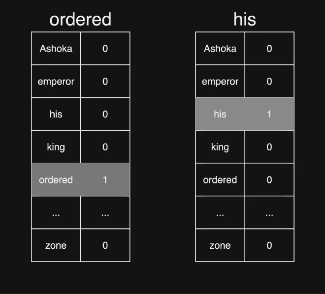
After creating a vector for every word in the vocabulary, we can move on to training the model. As an example, let’s take the vectors representing the words ordered and his. Through the input layer, the vector values enter the neural network, with a dedicated weight for each input. The values pass through the various neurons and layers, and we get output of the same size as the vector representing a word, in our case, 5000. The entry with the highest value will be the neural network’s prediction. Using a loss function, we will compare the prediction with the target word, adjust the neurons’ weights and biases (backpropagation), and repeat this several times.
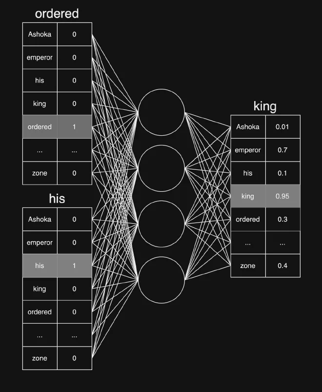
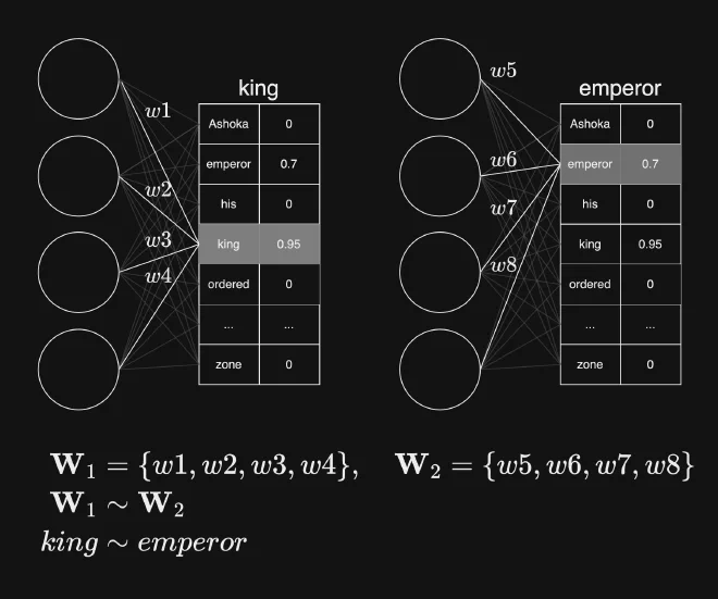
What happens when we have words with similar meanings? For example, we can associate the word “king” with the word pair “ordered, his”, but also the word “emperor”. In practice, when we feed the word pair “ordered, his” into the model, the weights leading to the output layer will be very close for “king” and “emperor”:
Python #
Step One - Importing Libraries #
Before we can start creating our Word2Vec model, we first need to import the libraries we will use.
import pandas as pd
import numpy as np
import matplotlib.pyplot as plt
import matplotlib.cm as cm

import gensim
from gensim.models import Word2Vec
from gensim.utils import simple_preprocess
import nltk
from nltk.corpus import stopwords

from sklearn.decomposition import PCA
from sklearn.cluster import KMeans
Step Two - Dataset #
The next step is to import our dataset. A few years ago, Amazon released its product review history; you can choose a dataset that interests you here. I chose meta_Electronics, which contains 178 million records and is 660MB in size.
df = pd.read_json("reviews_Cell_Phones_and_Accessories_5.json", lines=True)
df.shape
(194439, 9)
df.head()
| summary | overall | reviewText | helpful | reviewerName |
|---|---|---|---|---|
| Looks Good | 4 | They look good and stick good! I just don’t li… | [0, 0] | christina |
| Really great product. | 5 | These stickers work like the review says they … | [0, 0] | emily l. |
| LOVE LOVE LOVE | 5 | These are awesome and make my phone look so st… | [0, 0] | Erica |
| Cute! | 4 | Item arrived in great time and was in perfect … | [4, 4] | JM |
| leopard home button sticker for iphone 4s | 5 | awesome! stays on, and looks great. can be use… | [2, 3] | patrice m rogoza |
As you can see, our dataset contains 9 columns and about 200,000 records. Each record includes identifying information about the reviewer, the review text (reviewText), and the review rating. We want to implement the sentence completion problem using reviewText. The result will be a Word2Vec model.
df.loc[0, 'reviewText']
"They look good and stick good! I just don't like the rounded shape because I was always bumping it and Siri kept popping up and it was irritating. I just won't buy a product like this again"
Step Three - Preprocessing #
Gensim is an open-source library designed for unsupervised problems in natural language processing. Its name is short for Generate Similar, which already gives us an idea of its purpose: extracting understanding from context using texts. In the next step, we will use it to preprocess all the reviews.
For each record, the gensim.utils.simple_preprocess function performs three operations: it separates each word into its own entry, updates the entries to lowercase, and removes words that are too short (2 letters) or too long (over 15 letters). We can change its settings, but I decided to stick with the defaults.
review_text = df['reviewText'].apply(simple_preprocess)
review_text[0]
['good',
  'just',
  'don',
  'like',
  'the',
  'rounded',
  'shape',
  'because',
  'was',
  'always',
  'bumping',
  'it',
  'and',
  'siri',
  'kept',
  'popping',
  'up',
  'and',
  'it',
  'was',
  'irritating',
  'just',
  'won',
  'buy',
  'product',
  'like',
  'this',
  'again']
So now we have a Series in which each record contains a customer review. Each review is also split by word into a Series. Can you spot anything strange? We have quite a few stopwords. They are not relevant to our model; after all, we want to understand relationships between words. Stopwords contribute more to structure and syntax than to the context of words.
We used the NLTK library to get a list of English stopwords.
# Download the set of stop words the first time
nltk.download('stopwords')

# Load the stop words
stop_words = list(stopwords.words('english'))
stop_words[:10]
[nltk_data] Downloading package stopwords to
[nltk_data]     /home/ofir.linux/nltk_data...

['i', 'me', 'my', 'myself', 'we', 'our', 'ours', 'ourselves', 'you', "you're"]
Now that we have a list of stopwords, we will remove stopwords from our dataset. How? We will go through every row in review_text and keep a Series containing only the words that are not in stop_words.
filtered_sentences = review_text.apply(lambda sentence: [word for word in sentence if word not in stop_words])
filtered_sentences[0]
['look',
'good',
'stick',
'good',
'like',
'rounded',
'shape',
'always',
'bumping',
'siri',
'kept',
'popping',
'irritating',
'buy',
'product',
'like']
Step Four - Creating a Gensim Model #
Now that we have a basic dataset with enough records, we will define a Gensim model.
The models.Word2Vec function takes 3 parameters:
window- The context window size: the number of words we will feed into the model before and after the target word. For example, in the sentence the cat sat on the mat, if the word we are focusing on is “on” and the window is 2, the context fed into the model will be [“cat”, “sat”, “the”, “mat”].min_count- A threshold setting the minimum number of occurrences of words in the dataset. Words that appear fewer times than this threshold will not be taken into account.workers- The number of threads used while training the model. The model is trained on the computer’s local CPU.
We can also set the epochs. However, I decided to stick with the default of five passes over the dataset.
model = Word2Vec(
    window=10,
    min_count=2,
    workers=4,
)
After defining a model, we need to define its vocabulary. Gensim needs to know the words in advance to allocate storage space before training the model. The build_vocab function takes two parameters:
filtered_sentences- Our dataset on which we will train the model, after basic preprocessing.progress_per- Displaying processing progress.
model.build_vocab(filtered_sentences, progress_per=1000)
The two letters "wv" stand for Word Vectors: the word itself and its vector representation in the space.
model.wv.index_to_key[:10]
['phone',
  'case',
  'one',
  'like',
  'great',
  'use',
  'screen',
  'good',
  'battery',
  'would']
Step Five - Training #
We have reached my favorite stage: training the model. We will use the model.train function to start training the model. Let’s explore the parameters the function takes:
review_text- Our dataset on which we will train the model.total_examples- The number of sentences inreview_text. We will get this usingmodel.corpus_count.epochs- The number of times the model will iterate overreview_textduring training, usingmodel.epochs.
model.train(
    review_text,
    total_examples=model.corpus_count,
    epochs=model.epochs
)
(39455685, 83868975)
Yes! The model was trained successfully. Wait, what does “(39455685, 83868975)” mean? The first entry represents the total number of words the model processed during training: 39,455,685. The second entry represents the number of words if we had not restricted the model (total_examples): 83,868,975.
model.save("./word2vec-amazon-cell-accessories-reviews-short.model")
Now that we have a trained model, we can do a variety of things with it.
Step Six - Validation #
After training the model, there is an obvious next step: test it! I chose to test the model in two main ways:
- Finding words close to a given word -
most_similartakes a word and shows us a sorted list of nearby words, along with their semantic similarity scores from 0 to 1. - Comparing two words -
similaritytakes two words and returns their semantic similarity score from 0 to 1.
I noticed something interesting: our model identifies semantic similarity between synonyms. For example, for the word “bad”, the model estimated a similarity of 58% for the words “ok” and “okay”. This tells us that the dataset is small and that we should expand it. Regardless, the scores are relatively low, which also indicates a need to expand it.
model.wv.most_similar("bad")
[('terrible', 0.7134353518486023),
  ('horrible', 0.6528913378715515),
  ('good', 0.6117088198661804),
  ('poor', 0.5842180252075195),
  ('ok', 0.5830951929092407),
  ('okay', 0.5794284343719482),
  ('sad', 0.5713397860527039),
  ('awful', 0.5661174058914185),
  ('guess', 0.5649060010910034),
  ('sucks', 0.5634702444076538)]
model.wv.similarity(w1="cheap", w2="inexpensive")
0.5494996
model.wv.similarity(w1="great", w2="good")
0.75265694
Step Seven - Examining the Vectors #
We have a model, and we have a vocabulary. We have played around with it a little and seen semantic relationships between words. Let’s get a better idea of what the vectors look like, and then we will perform PCA.
How can we access the value of our first vector in the word embedding? As we learned earlier, our model object contains the vectors: model.wv. Through index_to_key, we can access the word, and through vectors, we can access its representative vector.
first_word = model.wv.index_to_key[0]
first_vector = model.wv.vectors[0]

print(f"The first word is: {first_word}")
print(f"The corresponding vector is: {first_vector}")
The first word is: phone
The corresponding vector is: [ 0.5008796   0.15167381  2.333319    0.10688468 -1.8840703  -1.6957991
  0.05495637  0.05827418  0.2887405  -1.5429118   0.7645639   1.5215374
  -1.0641086  -2.0851662   1.9897771   1.7530214  -1.4697678   1.203952
  -0.5528912   0.86333096  0.34154853  0.40921074  1.8353231  -0.70408404
  0.7073904   0.26164898 -0.49617675 -1.1880581  -1.7986948  -0.54001534
  -1.6011297  -0.71133554  0.06995012 -0.771902    1.0777777   0.54750687
  0.4895541  -0.19904068 -0.75305825  0.20286536 -0.12561971  0.6058311
  -1.7315526   0.21385051 -0.29921278  2.2685251   0.23338611  1.1759087
  -0.4928176   1.200081    0.16036424  1.461912   -0.27610686  0.78729796
  -1.3324577  -2.002154   -1.886145   -1.2060144   0.09603836  0.441084
  -0.84192204  1.3879699  -1.5583698  -2.1753058   1.8789396   1.8851941
  2.532747   -3.5517168   4.300643    1.8870016  -0.13734312 -1.1338986
  0.37865153 -3.2530427   0.2187101   0.08842526 -0.7187293  -1.6173351
  -2.2799978  -2.930807    1.586075    1.0674981   0.0357586  -0.2196174
  0.55386424  0.47894716  0.58673614 -1.2975037  -2.2414744   0.854725
  0.24780588 -1.8748467   1.1259404  -0.6548109   0.7133601  -0.99056697
  -2.082928   -1.9393501  -0.1883115   1.9074923 ]
Let’s dig a little deeper and display the vector on a graph:
plt.figure(figsize=(12, 4))
plt.plot(first_vector)
plt.title(f"Vector for Word: '{first_word}'")
plt.xlabel('Dimension')
plt.ylabel('Value')
plt.show()
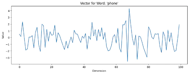
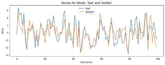
Even though our model has 100 dimensions, how were we able to visualize it? For each dimension (represented by a separate entry in the first_vector array), we checked its corresponding value. Then we created a basic plot. To explore further, it would be interesting to look at vectors of words with the same meaning, so we could see visually why the model decided they were close.
bad_vector = model.wv['bad']
terrible_vector = model.wv['terrible']

plt.figure(figsize=(12, 4))

plt.plot(bad_vector, label="bad")
plt.plot(terrible_vector, label="terrible")

plt.title("Vectors for Words: 'bad' and 'terrible'")
plt.xlabel('Dimension')
plt.ylabel('Value')
plt.legend()
plt.show()
Step Eight - Performing PCA and Plotting the Results #
PCA, or Principal Component Analysis, reduces the number of dimensions while aiming to preserve most of the information. We will use PCA to visualize the relationships between words.
As we saw earlier, each vector in our model has 100 dimensions. Each dimension represents a certain meaning for each word, its use in a sentence, and the relationship between words. PCA lets us convert these relationships into graphs with dimensions we can understand.
common_words = model.wv.index_to_key[:250]
common_vectors = model.wv[common_words]

pca = PCA(n_components=2)
pca_result = pca.fit_transform(common_vectors)

pca_result[:10]
array([[ -2.8586824 ,  -2.0252922 ],
        [-10.519664  ,  -0.06634452],
        [  0.4119802 ,   2.6990404 ],
        [ -3.819451  ,  -1.0890281 ],
        [ -1.0121241 ,   0.6645675 ],
        [  3.1565413 ,  -2.0301502 ],
        [ -9.929559  ,   1.2011172 ],
        [ -2.5529263 ,   0.71880364],
        [ 10.047557  ,  -0.7733079 ],
        [ -0.8474419 ,   0.74553484]], dtype=float32)
pca_df = pd.DataFrame(pca_result, columns=['x_values', 'y_values'])
pca_df['word'] = common_words

pca_df.head()
| word | y_values | x_values | index |
|---|---|---|---|
| phone | -2.025292 | -2.858682 | 0 |
| case | -0.066345 | -10.519664 | 1 |
| one | 2.699040 | 0.411980 | 2 |
| like | -1.089028 | -3.819451 | 3 |
| great | 0.664567 | -1.012124 | 4 |
| … | … | … | … |
| drop | 0.963806 | -8.024269 | 245 |
| said | 4.825479 | -0.982296 | 246 |
| chargers | 0.804604 | 11.564008 | 247 |
| left | -3.246815 | 2.390023 | 248 |
| card | -1.351355 | -1.503416 | 249 |
The code we wrote has 3 main parts:
- Word vectors - We access the 250 most frequent words in the model;
index_to_keyis sorted from the most frequent word downward. - Performing PCA - We used the sklearn library, whose full name is scikit-learn. This library provides a toolkit of efficient and simple tools (depending on whom you ask) for analyzing data and building models.
Usingn_components, we defined the number of dimensions we wanted to get from PCA. Then we obtainedpca_df, which contains the word along with its representation on the x and y axes. - Assembling the df - Now that we have each vector’s “reduced” value along both axes in the
pca_resultarray, we combine them into a single df namedpca_df.
Let’s see what pca_df looks like on a graph.
plt.figure(figsize=(12, 8))
plt.scatter(pca_df['x_values'], pca_df['y_values'])

for i, word in enumerate(pca_df['word']):
    plt.annotate(word, (pca_df['x_values'].iloc[i], pca_df['y_values'].iloc[i]))

plt.xlabel('First Principal Component')
plt.ylabel('Second Principal Component')
plt.title('Word2Vec Word Embeddings Visualized with PCA')
plt.show()
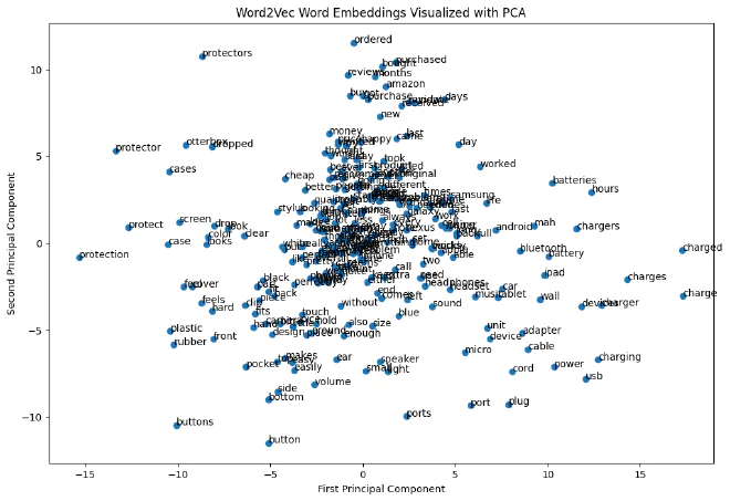
All right, now we have a graph showing the word embedding we created. The natural next step is to create clusters from it.
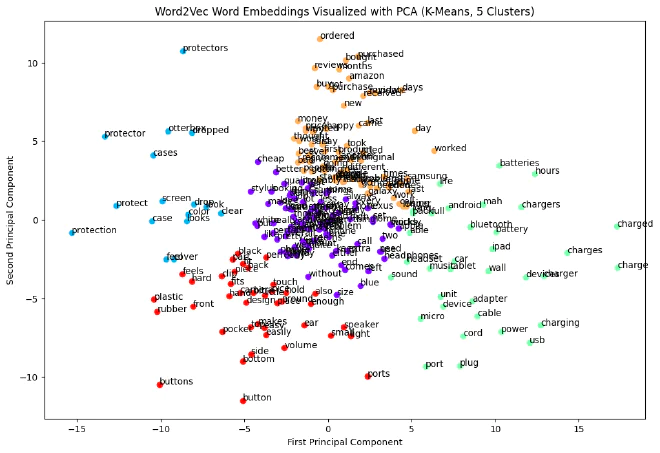
First, we need to create our clusters. Wait, what does that even mean? Clusters are used in unsupervised problems when we want to divide the dataset into K parts (in our code, num_clusters), provided that they overlap in the same area of the graph.
# Number of clusters
num_clusters = 5

# Fit K-means
kmeans = KMeans(n_clusters=num_clusters, n_init=10)
pca_df['cluster'] = kmeans.fit_predict(pca_result)
We created a kmeans object with 5 parts. Then, using the fit_predict function, we divided the pca_result array into 5 parts.
The next step is to display the nice clusters we made on a graph. Since I think it looks better to display each cluster in a different color, we will define a colors array containing as many different colors as we have clusters.
Then, for each cluster, we will define a scatter plot in a shared figure and add labels with the words.
I recommend spending a few minutes looking at the words and clusters we ended up with.
plt.figure(figsize=(12, 8))

colors = cm.rainbow(np.linspace(0, 1, num_clusters))

for cluster, color in zip(range(num_clusters), colors):
    cluster_df = pca_df[pca_df['cluster'] == cluster]
    plt.scatter(cluster_df['x_values'], cluster_df['y_values'], color=color)

    for i, word in cluster_df['word'].items():
        plt.annotate(word, (cluster_df['x_values'].loc[i], cluster_df['y_values'].loc[i]))

plt.xlabel('First Principal Component')
plt.ylabel('Second Principal Component')
plt.title(f'Word2Vec Word Embeddings Visualized with PCA (K-Means, {num_clusters} Clusters)')
plt.show()
I hope you learned a thing or two. See you in the next article! 😀