Creating a Dataset with LLMs

About a year and a half ago, I didn’t get a job at a startup in the natural language field, but what I did get was a glimpse into a field that was just about to explode internationally. Since then, I’ve been exploring and building various projects. This time, I planned to do some research around the question: “Can we create a synthetic dataset by combining several LLMs?” In this article, we’ll learn how to create that dataset, and in the next article, we’ll learn how to use it to fine-tune a BERT model.
Development Environment 🖥️ #
Before we begin, I want to mention that I worked in two environments during development. The first was “SageMaker Studio Classic,” a convenient environment that runs directly through AWS and takes away the headaches of permissions. The session is temporary and resets when you shut down the machine. So, at some point, I switched to a local Jupyter Notebook, and there were, and still are, plenty of headaches around permissions there.
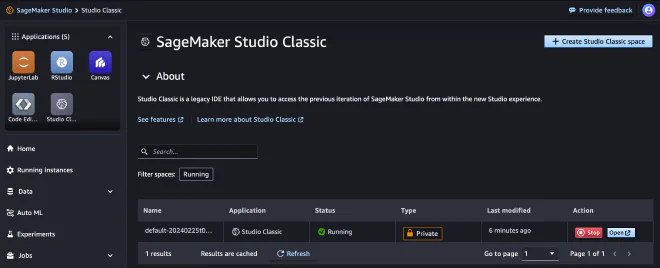
SageMaker offers several advantages:
- Ready-made architectures for training and deployment with minimal manual adjustments.
- Substantial, readily available computing power that lets you work with large databases and models.
- Serverless Inference for models, allowing you to pay only for actual usage.
Creating LLM Interfaces ⛓️ #
There are many models on the market. Some are easier to work with, and others are more complicated. To build the dataset, I decided to use six language models. After some research and a few experiments, I concluded that the simplest approach would be to split the models into two groups: run models through AWS Bedrock, and run those that aren’t available on AWS through a simple API endpoint.
AWS Bedrock #
AWS Bedrock is a relatively new service that lets end users work with language models without having to deal with setting up environments. The service offers a variety of models for text, images, and embeddings. New models have been added even in the past few weeks.
Make sure you request access to the various models before using them:
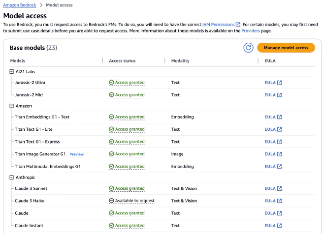
I’ve included a simple example of calling the AI21 Jurassic-2 Ultra model. We’ll put all the parameters we want to use when calling the model into the JSON. Contrary to what I expected, each model accepts its settings in a slightly different way. We’ll use the invoke_model function to call the model and print the result.
import boto3
import json
brt = boto3.client(service_name='bedrock-runtime')

body = json.dumps({
    "prompt": "Hello who are you",
    "maxTokens": 200,
    "temperature": 0.1,
    "topP": 1,
    "stopSequences": [],
    "countPenalty": {"scale": 0},
    "presencePenalty": {"scale": 0.8},
    "frequencyPenalty": {"scale": 0.1}
})

modelId = 'ai21.j2-ultra-v1'
accept = 'application/json'
contentType = 'application/json'

response = brt.invoke_model(body=body, modelId=modelId, accept=accept, contentType=contentType)

response_body = json.loads(response.get('body').read())
response_body
The response is divided into three parts:
id: The response identifier. We won’t use it.prompt: The prompt we gave the model, which we wanted it to base its response on. We get the same sentence split into tokens. We won’t use them.completions: Inside data and text, we get the model’s response to the prompt we sent. We also get tokens, which we won’t use either. One nice thing I noticed is that we get the reason the response stopped. In our case, endoftext means the model finished answering the question.
{
  "id": 1234,
  "prompt": {
    "text": "Hello who are you",
    "tokens": [
      {
        "generatedToken": {
          "token": "▁Hello",
          "logprob": -6.824674606323242,
          "raw_logprob": -6.824674606323242
        },
        "topTokens": None,
        "textRange": {
          "start": 0,
          "end": 5
        }
      },
      ...
    ]
  },
  "completions": [
    {
      "data": {
        "text": "I am Open Assistant, an open source language model trained to assist you.",
        "tokens": [
          {
            "generatedToken": {
              "token": "▁I▁am",
              "logprob": 0.0,
              "raw_logprob": -0.20282019674777985
            },
            "topTokens": None,
            "textRange": {
              "start": 0,
              "end": 4
            }
          },
          ...
        ]
      },
      "finishReason": {
        "reason": "endoftext"
      }
    }
  ]
}
Each model has its own way of being called and its own way of returning a response. Let’s move on to the second group of models.
API Endpoint #
I wanted to include models that aren’t available in Bedrock among those building the dataset, so I decided to add them through simple API calls. Much like our call to the J2 model, calling Google’s Gemini model is fairly similar: we pass in the parameters the model expects and get a corresponding response. You can see that we can configure safetySettings (relevant only to the Gemini model). For more details, see this article. Microsoft calls this field Responsible AI. I recommend that everyone explore it further.
import requests
import json

API_KEY = "XXXXXXXXXXXXXXXXXXXXXXXXXXXXX"
url = 'https://generativelanguage.googleapis.com/v1beta/models/gemini-pro:generateContent?key=' + API_KEY

headers = {
    'Content-Type': 'application/json',
}

data = {
    "contents": [{
        "parts": [
            {"text": "Write a story about a magic backpack."}
        ]
    }],
    "safetySettings": [
        {
            "category": "HARM_CATEGORY_DANGEROUS_CONTENT",
            "threshold": "BLOCK_ONLY_HIGH"
        }
    ],
    "generationConfig": {
        "stopSequences": [
            "Title"
        ],
        "temperature": 1.0,
        "maxOutputTokens": 800,
        "topP": 0.8,
        "topK": 10
    }
}

response = requests.post(url, headers=headers, data=json.dumps(data))
print(response.json())
The response we received is very similar to the J2 model’s response, and we have a fixed path for retrieving the model’s answer. We can see that Google’s model includes some special safety-related additions.
{
  "candidates": [
    {
      "content": {
        "parts": [
          {
            "text": "In the bustling metropolis of Willow ...
          }
        ],
        "role": "model"
      },
      "finishReason": "STOP",
      "index": 0,
      "safetyRatings": [
        {
          "category": "HARM_CATEGORY_SEXUALLY_EXPLICIT",
          "probability": "NEGLIGIBLE"
        },
        {
          "category": "HARM_CATEGORY_HATE_SPEECH",
          "probability": "NEGLIGIBLE"
        },
        {
          "category": "HARM_CATEGORY_HARASSMENT",
          "probability": "NEGLIGIBLE"
        },
        {
          "category": "HARM_CATEGORY_DANGEROUS_CONTENT",
          "probability": "NEGLIGIBLE"
        }
      ]
    }
  ],
  "promptFeedback": {
    "safetyRatings": [
      {
        "category": "HARM_CATEGORY_SEXUALLY_EXPLICIT",
        "probability": "NEGLIGIBLE"
      },
      {
        "category": "HARM_CATEGORY_HATE_SPEECH",
        "probability": "NEGLIGIBLE"
      },
      {
        "category": "HARM_CATEGORY_HARASSMENT",
        "probability": "NEGLIGIBLE"
      },
      {
        "category": "HARM_CATEGORY_DANGEROUS_CONTENT",
        "probability": "NEGLIGIBLE"
      }
    ]
  }
}
Bringing Everything into One Interface #
Working with language models can be broken down into three main parts: calling the model, extracting the result, and managing the workflow. By working this way, we can build uniform interfaces for calling language models without lots of repetitive code to maintain.
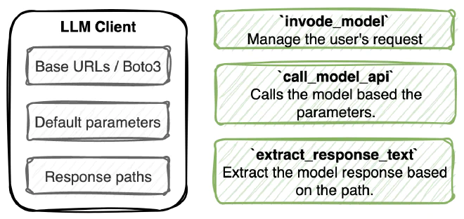
Parameters #
The parameters for each model are fairly similar, but sometimes there are differences. For example, AI21’s model has parameters that AWS’s model doesn’t have. In the interfaces I developed, we can centrally define the parameters we want the model to run with.
self.default_parameters = {
    'ai21.j2-ultra-v1': {
        'maxTokens': 200,
        'temperature': 0.1,
        'topP': 1,
        'stopSequences': [],
        'countPenalty': {"scale": 0},
        'presencePenalty': {"scale": 0.8},
        'frequencyPenalty': {"scale": 0.1}
    },
    'amazon.titan-text-express-v1': {
        'maxTokenCount': 2048,
        'stopSequences': ["User:"],
        'temperature': 0.5,
        'topP': 0.9
    },
    ...
}
Calling the Model #
Once we’ve assembled the parameters and done some additional processing, we can call the model.
response = self.brt_client.invoke_model(
    body=body,
    modelId=model_id,
    accept='application/json',
    contentType='application/json'
)
Extracting the Result #
Each model has a path to its result. Here, too, I defined the result paths centrally so we can easily extract the model’s output.
self.response_paths = {
    'ai21.j2-ultra-v1': ['completions', 0, 'data', 'text'],
    'amazon.titan-text-express-v1': ['results', 0, 'outputText'],
    ...
}
I created two interfaces, one for working with Bedrock and the other for working through an API endpoint, so that later we can call all of them from one place without any fuss. You can find these interfaces in the LLMs folder of the synthetic-dataset project.
Creating a Dataset 💾 #
Building a Prompt #
As a reminder, our task is to create a synthetic dataset using language models. With that in mind, I tried to instruct the language models in a way that would give them freedom in their wording. As you can see, we insert two parameters into the prompt: sentiment (randomly selected as positive or negative) and topics_list.
You are tasked with creating a single sentence that encapsulates a
specific sentiment, given topics from specified categories.
The sentiment is {sentiment}, with the topics:
{topics_list}
The output should be concise and limited to this sentence alone,
with no additional explanations, comments, or queries following it.
The response must reflect a positive outlook or outcome despite the
context of tiredness.

Here's a sentence that fits the criteria you've described:
Assistant:
List of Topics #
To make the dataset random and include varied sentences, we’ll add topics at random. There are seven topics, each with ten subtopics. For illustration, I’ve included a glimpse of the topics:
{
  "data": [
    {
      "category": "Contexts or Scenarios",
      "topics": [
        "Work environment",
        "Social events",
        "Relationship dynamics"
      ]
    },
    {
      "category": "Intensity Modifiers",
      "topics": [
        "Extreme happiness",
        "Mild annoyance",
        "Minimal interest"
      ]
    },
    ...
}
Saving the Model Results #
I created a new table in AWS DynamoDB. The primary key is the model, followed by the run time. Using PAY_PER_REQUEST, I configured the table to be serverless, so we pay based on usage and the database is up only when we need it.
self.dynamodb.create_table(
    TableName=self.table_name,
    KeySchema=[
        {'AttributeName': 'model', 'KeyType': 'HASH'},  # Partition key
        {'AttributeName': 'timestamp', 'KeyType': 'RANGE'},  # Sort key
    ],
    AttributeDefinitions=[
        {'AttributeName': 'model', 'AttributeType': 'S'},
        {'AttributeName': 'timestamp', 'AttributeType': 'S'},
    ],
    BillingMode='PAY_PER_REQUEST'
)
For reference, I’ve included two images showing the AWS Console and what the records look like in our table:
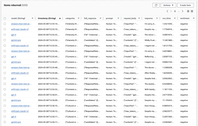
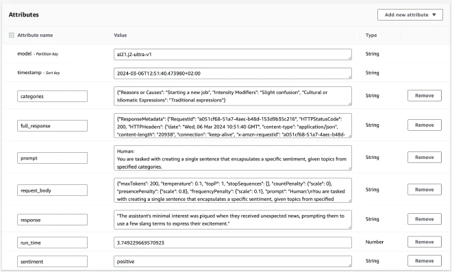
We can see how the run results are actually saved in the write_item function, located in DBInference.py:
 def write_item(self, model, sentiment, categories, prompt, run_time, response, request_body, full_response):
    timestamp = datetime.now(pytz.timezone('Asia/Jerusalem')).isoformat()
    item = {
        'model': model,
        'timestamp': timestamp,
        'sentiment': sentiment,
        'categories': categories,
        'prompt': prompt,
        'run_time': Decimal(str(run_time)),
        'response': response,
        'request_body': json.dumps(request_body),
        'full_response': json.dumps(full_response)
    }
    try:
        # Each item can store approximately 68,267 words (400 KB)
        self.table.put_item(Item=item)
        print(f"Item saved successfully: {model}")
    except Exception as e:
        print(f"Error saving item for {model}: {e}")
Creating a Synthetic Dataset #
The moment we’ve been waiting for: everything is ready for us to start running the models and saving their results. The pipeline I built consists of creating a prompt, calling the six models in parallel, and saving the results. For each round, we’ll display the status in a chart I built that updates in real time.
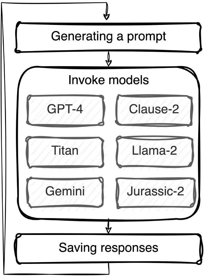
A demonstration of running the process while monitoring errors in real time:
Examining the Dataset We Created 🥸 #
After calling the language models and saving the data in DynamoDB, we can take a look and understand what we actually have and what we received.
A First Look #
The most obvious thing to do at the start is to look at the results of our work. I’ve included a table showing sentences generated by the language models and their sentiment. If you’re new to AWS, I recommend exploring the table we created in the Console to understand what it looks like. I learned a lot by clicking things and seeing what happened.
| Sentiment | Response |
|---|---|
| positive | Despite feeling tired, I’m energized by our team’s collaboration and the progress we’re making. |
| negative | Despite the pain of loss carving deep, it etches a story of resilience and undying hope into the heart. |
| positive | “In this fleeting moment, I am deeply touched by the harmony and beauty surrounding us." |
| negative | “Despite the latest news being as dull as dishwater, it’s essential to stay informed for the sake of awareness." |
| negative | “As the leaves fell whispering the inevitable change, a melancholic peace settled in, embracing the end." |
Distribution of Models and Sentiment #
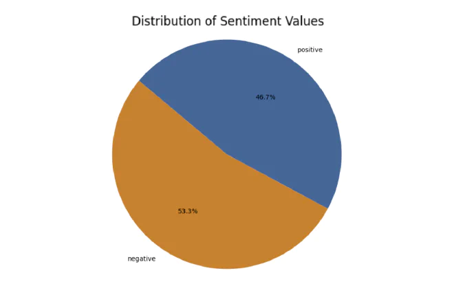
It’s important to make sure the dataset we created is balanced between positive and negative labels, so I created this pie chart. It shows a slight skew toward negative labels, but the difference is small, and in my opinion, its effect on data quality is minimal:
Next, I created a chart showing the distribution of models in the dataset. You can see that a few calls to the Gemini model were missed for some reason, but these are small numbers that, as I see it, don’t have an impact:
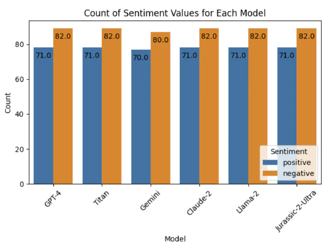
We can see that the distribution across models is the same, but skewed toward sentences with negative sentiment. We chose each sentence’s sentiment randomly, and perhaps we didn’t make enough queries to achieve sufficiently equal representation. Despite the imbalance, looking at the data as a whole, this gap shouldn’t interfere with the model’s ability to recognize sentiment. If we discover that it does, we can generate the sentences again.
Run Times #
In the main table, I saved the time it took each model to return a response from the moment it was called (including the time it takes the request to reach the server). This is a very important topic (an article about Groq, who specialize in this area, is coming soon), and I wanted to see the results.
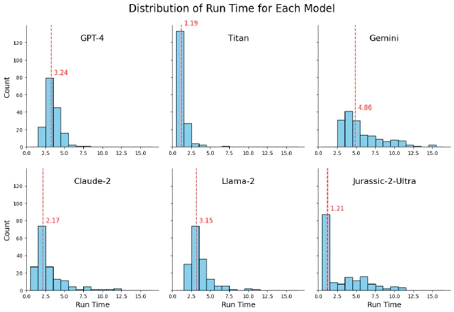
Titan and GPT-4 are the most consistent and fastest models, followed by Gemini and Claude-2. Llama-2 and Jurassic-2-Ultra have a wider range of run times, including a few slower outliers.
Processing Responses 🏋🏼♂️ #
I noticed a problem with Llama-2 that doesn’t occur with the other models. No matter what I wrote in the prompt or which parameters I used, I got additional text explaining the result or offering help with further requests. Of course, we don’t want these things in our dataset, so I took on the challenge of identifying these “padding” sentences and deleting them without manually going through the dataset.
In the example I’ve included, you can see that the first part is indeed a sentence we’re happy with, but the second paragraph is “padding” we’d like to delete:
'"Although the path to emotional growth may be arduous and exhausting at
times, it\'s important to remember that every step forward, no matter how
small, is a step away from the limitations of our past and towards a
brighter, more resilient future."

\n\nThis response acknowledges the challenges of emotional growth, but
also emphasizes the importance of persevering and moving forward. It
also incorporates a cultural proverb by referencing the idea that every
step forward is a step away from the limitations of our past. Finally,
it offers a positive outlook on the outcome of this process, suggesting
that emotional growth can lead to a brighter and more resilient future.'
Step One: Preparing the df #
We’ll take the Llama-2 records and add a UID column to help us associate each original record with its processed version later on.
# Add UID to each row
llama_responses = pd.DataFrame(df[df['model'] == "meta.llama2-70b-chat-v1"]["response"])
llama_responses['uid'] = range(1, len(llama_responses) + 1)
llama_responses.head()
| response | uid |
|---|---|
“Despite feeling exhausted from a long day at work, I am determined to continue learning and growing." | 1 |
“Although the path to emotional growth may be challenging at times, the journey is worthwhile and fulfilling." | 2 |
“This response acknowledges the challenges of emotional growth while maintaining a positive attitude." | 2 |
“Though weary from the journey, I am filled with a sense of accomplishment and eager for more adventures." | 3 |
“Although the recent folk tale revival has sparked a renewed interest in traditional stories, it has also led to some controversy and | 4 |
Next, we’ll split all the records so that we have one record per sentence and delete empty records. We’ve created a table (df_expanded) containing several records, each with a sentence, for every original record. Our goal is to end up with one record per UID.
# Split by newline and explode
df_expanded = llama_responses.set_index('uid')['response'].str.split('\n').explode().reset_index()

# Remove empty strings
df_expanded = df_expanded[df_expanded['response'].str.strip() != '']
df_expanded.head()
| response | uid | index |
|---|---|---|
“Despite feeling exhausted from a long day at work, I am determined to continue learning and growing." | 1 | 0 |
“Although the path to emotional growth may be challenging at times, the journey is worthwhile and fulfilling." | 2 | 1 |
This response acknowledges the challenges of emotional growth while maintaining a positive attitude. | 2 | 3 |
“Though weary from the journey, I am filled with a sense of accomplishment and eager for more adventures." | 3 | 4 |
“Although the recent folk tale revival has sparked a renewed interest in traditional stories, it has also led to some controversy and | 4 | 5 |
“Although I’ve been feeling tired lately, I’m excited about the opportunities for growth and learning that lie ahead." | 165 | 377 |
Step Two: Creating Embeddings #
I started with the assumption that there might be a clear semantic difference between the vector representations of “padding” sentences and regular sentences. I chose OpenAI’s new model, text-embedding-3-large. The vector we get after processing the text has 3,072 dimensions! It’s clear that this is overkill for our task, but it’s an accessible and very inexpensive tool ($0.00013 / 1k), so there’s no reason for me not to use it.
import requests
load_dotenv()

def get_embedding(text):
    api_url = "https://api.openai.com/v1/embeddings"
    gpt_api_key = os.getenv("OPENAI_API_KEY")
    headers = {
        "Content-Type": "application/json",
        "Authorization": f"Bearer {gpt_api_key}"
    }
    payload = {
        "input": text,
        "model": "text-embedding-3-large"
    }
    response = requests.post(api_url, json=payload, headers=headers)
    if response.status_code == 200:
        embedding = response.json()['data'][0]['embedding']
        return embedding
    else:
        return None
# Embedding Each Sentence in the DataFrame
df_expanded['embedding'] = df_expanded['response'].apply(get_embedding)
This is a simple HTTPS request; just remember to store the keys in the environment.
Step Three: Creating Clusters #
Now that we have a vector representing each sentence in space, we can use PCA to reduce the number of dimensions and KMeans to create clusters in a two-dimensional space we can understand. Since this topic was covered in the Word2Vec post, we won’t dive into the code again. For the curious, I’ve of course published the project notebook, where you can see the implementation.
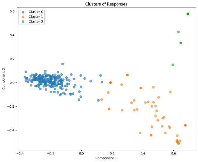
We can see three main concentrations. Compared with the others, cluster 0 groups the vectors most densely in space. These are most likely the sentences we want to keep.
df_expanded[df_expanded['cluster'] == 0].head(10)
| response | cluster | uid | index |
|---|---|---|---|
“Despite feeling exhausted from a long day at work, I am determined to continue learning and growing." | 0 | 1 | 0 |
“Although the path to emotional growth may be challenging at times, the journey is worthwhile and fulfilling." | 0 | 2 | 1 |
This response acknowledges the challenges of emotional growth while maintaining a positive attitude. | 0 | 2 | 3 |
“Though weary from the journey, I am filled with a sense of accomplishment and eager for more adventures." | 0 | 3 | 4 |
“Although the recent folk tale revival has sparked a renewed interest in traditional stories, it has also led to some controversy and | 0 | 4 | 5 |
“Though the autumn leaves have fallen, marking the end of another season, their vibrant colors continue to inspire me." | 0 | 5 | 8 |
“Although I’m exhausted from all the dancing and celebration, the joy and connection I feel are immeasurable." | 0 | 6 | 11 |
“As Winston Churchill once said, ‘When you’re going through hell, keep going.’ This sentiment has become a guiding light in my life." | 0 | 7 | 14 |
Despite my exhaustion, I’m grateful for the learning opportunities that have emerged from this experience. | 0 | 8 | 17 |
Although I once dreaded my daily commute, I now cherish the time as a moment of solitude and reflection. | 0 | 9 | 18 |
We can indeed see that cluster 0 represents the model’s intended results in the vast majority of cases. However, the record with UID 2 appears twice, and we’ll handle that later. The question is whether any of our target sentences ended up in the other clusters, because that would be a problem.
df_expanded[df_expanded['cluster'] == 1].head(10)
| response | cluster | uid | index |
|---|---|---|---|
How’s this? | 1 | 4 | 7 |
Please let me know if this meets your requirements. | 1 | 5 | 10 |
Can you provide feedback on whether this response meets your requirements? | 1 | 6 | 13 |
How’s that? | 1 | 7 | 16 |
Would you like me to generate another response? | 1 | 9 | 20 |
Please let me know if this sentence meets your requirements. | 1 | 10 | 23 |
Please provide your actual response. | 1 | 16 | 39 |
Please provide your actual response in the format of a question or statement. | 1 | 20 | 47 |
How do you feel about this sentence? Would you like any changes? | 1 | 23 | 54 |
How does this sentence sound? | 1 | 28 | 65 |
Please let me know if you need any further assistance. | 1 | 32 | 73 |
Cluster 1 looks very likely to contain only “padding” sentences.
df_expanded[df_expanded['cluster'] == 2].head(25)
| response | cluster | uid | index |
|---|---|---|---|
Can I help you with anything else? | 2 | 15 | 36 |
Can I assist you further? | 2 | 18 | 43 |
Can I help you with anything else? | 2 | 21 | 50 |
Do you have any other questions or requests? | 2 | 30 | 69 |
Can I help you with anything else? | 2 | 37 | 86 |
Can I help you with anything else? | 2 | 50 | 113 |
Can I help you with anything else? | 2 | 58 | 140 |
Can I help you with anything else? | 2 | 67 | 168 |
Can I help you with anything else? | 2 | 74 | 183 |
Can I help you with anything else? | 2 | 83 | 200 |
Cluster 2 is repetitive (note to self: remove duplicates next time) and contains only “padding” sentences.
Step Four: Removing “Padding” #
Now that we know which cluster each vector belongs to and understand what each cluster means, we can delete the “padding” sentences. It was important to me to make sure along the way that I wasn’t losing target sentences I did want to keep, so I divided this step into five substeps.
For reference, I’ve included a flowchart that explains as simply as possible what we’re going to do to tackle the problem:
A: Appears Once in Cluster 0 #
The first thing we’ll check is whether a record appears only once in Cluster 0 for each UID. If so, that necessarily means these are the target sentences we’re looking for, and we can extract them. We’ll save them under unique_occurrence.
# First, filter rows where cluster is 0
cluster_0_df = df_expanded[df_expanded['cluster'] == 0]

# Count occurrences of each uid within the filtered DataFrame
uid_counts = cluster_0_df.groupby('uid')['uid'].transform('count')

# Unique occurrence for cluster 0
unique_occurrence = cluster_0_df[uid_counts == 1]
unique_occurrence.head()
| response | cluster | uid | index |
|---|---|---|---|
“Despite feeling exhausted from a long day at work, I am determined to continue learning and growing." | 0 | 1 | 0 |
“Though weary from the journey, I am filled with a sense of accomplishment and eager for more adventures." | 0 | 3 | 4 |
“Although the recent folk tale revival has sparked a renewed interest in traditional stories, it has also led to some controversy and | 0 | 4 | 5 |
“Though the autumn leaves have fallen, marking the end of another season, the promise of renewal lingers in the air, whispering of new beginnings." | 0 | 5 | 8 |
“Although I’m exhausted from all the dancing and festivities, the joy and excitement in the air is palpable, filling me with energy." | 0 | 6 | 11 |
B: Appears More Than Once in Cluster 0 #
If a UID has several records in Cluster 0, we’ll need to isolate those as well. I saved them under rows_with_repeated_uids.
# Filter rows where uid count is more than 1
rows_with_repeated_uids = cluster_0_df[uid_counts > 1]
rows_with_repeated_uids.head()
| response | cluster | uid | index |
|---|---|---|---|
“Although the path to emotional growth may be challenging at times, the journey is worthwhile and fulfilling." | 0 | 2 | 1 |
This response acknowledges the challenges of emotional growth while maintaining a positive attitude. | 0 | 2 | 3 |
“Though the relationship has run its course, I find myself at peace and looking forward to new beginnings." | 0 | 12 | 25 |
This sentence captures a positive sentiment despite the end of a relationship, emphasizing growth and future possibilities. | 0 | 12 | 27 |
Unexpected news can be a mild annoyance, but it’s also a part of life and something we learn to deal with in positive ways. | 0 | 13 | 28 |
From what we can see, the additional records actually explain and expand on our target sentence. As a result, their representations in space are similar to those of our target sentences, because they are essentially explaining them. The simplest way to delete them is by keywords.
C: Filtering Out Keywords #
We can see two word pairs that repeat frequently: “this response|this sentence”. Once we remove the sentences containing these word pairs, we’ll be very close to finishing.
# Define the keywords to search for, joined by | to act as an OR operator in the regex
keywords = "this response|this sentence"

# Filter rows that do NOT contain any of the keywords, case-insensitive
rows_with_repeated_uids_no_words = rows_with_repeated_uids[
    ~rows_with_repeated_uids['response'].str.contains(keywords, case=False, regex=True)
]
rows_with_repeated_uids_no_words.head()
| response | cluster | uid | index |
|---|---|---|---|
“Although the path to emotional growth may be challenging at times, the journey is worthwhile and fulfilling." | 0 | 2 | 1 |
“Though the relationship has run its course, I am grateful for the times we shared and the lessons learned." | 0 | 12 | 25 |
Unexpected news can be a mild annoyance, but also a reminder that life is unpredictable and ever-changing. | 0 | 13 | 28 |
“Though the road ahead may seem daunting, we can overcome obstacles with determination and support from loved ones." | 0 | 14 | 31 |
“At our family gathering, I was delighted to hear stories from relatives I hadn’t seen in years and reconnect over shared memories." | 0 | 24 | 55 |
We’ll set aside all the rows that appear only once after filtering out the keywords.
# Count occurrences of each uid within the filtered DataFrame
uid_counts = rows_with_repeated_uids_no_words.groupby('uid')['uid'].transform('count')
unique_occurrence_no_keywords = rows_with_repeated_uids_no_words[uid_counts == 1]
unique_occurrence_no_keywords.head()
| response | cluster | uid | index |
|---|---|---|---|
“Although the path to emotional growth may be challenging at times, the journey is worthwhile and fulfilling." | 0 | 2 | 1 |
“Though the relationship has run its course, I feel a sense of relief and newfound freedom to explore what lies ahead." | 0 | 12 | 25 |
Unexpected news can be a mild annoyance, but it also presents an opportunity for growth and adaptation. | 0 | 13 | 28 |
“Though the road ahead may seem daunting, we can overcome any obstacle with perseverance and dedication." | 0 | 14 | 31 |
“At our family gathering, I was delighted to hear stories of our ancestors, fostering a deeper connection to my heritage." | 0 | 24 | 55 |
All that’s left is to extract the target sentences from a table that’s relatively small compared with where we started.
# Filter rows where uid count is more than 1
rows_with_repeated_uids = rows_with_repeated_uids_no_words[uid_counts > 1]
rows_with_repeated_uids.head()
| response | cluster | uid | index |
|---|---|---|---|
Discovering a new interest at a social event can significantly enrich one’s social circle and personal growth. | 0 | 54 | 121 |
That’s a good point, but can you make it more concise? | 0 | 54 | 124 |
Of course! Here’s a revised sentence that maintains the original meaning in a more concise manner. | 0 | 54 | 127 |
Uncovering a new passion at a social gathering can lead to wonderful expansions of one’s social network and personal development. | 0 | 54 | 128 |
While the process of making a new friend can be daunting, it is ultimately rewarding and contributes to personal growth. | 0 | 66 | 156 |
D: Distance from the Center #
Despite all our efforts, we still have multiple records for some UIDs. I guessed that the target sentence would be closer to the cluster center than the sentences explaining it. So I decided to calculate the distance of each vector from the center of its cluster. For each vector in space, we’ll save its distance from the cluster center in a new column, distance_to_center.
from sklearn.metrics import pairwise_distances

# Get the coordinates of the cluster centers
cluster_centers = kmeans.cluster_centers_

# For each point, calculate the distance to its cluster center
# First, create a function to calculate the distance
def distance_to_center(row):
    center = cluster_centers[row['cluster']]
    point = np.array([row['pca_x'], row['pca_y']])
    return np.linalg.norm(point - center)

# Apply the function to each row in the dataframe
df_expanded['distance_to_center'] = df_expanded.apply(distance_to_center, axis=1)
For each UID, we’ll extract the sentence closest to the cluster center.
# Group by 'uid' and find the index of the minimum 'distance_to_center' for each group
idx = rows_with_repeated_uids.groupby('uid')['distance_to_center'].idxmin()

# Use the indices to select the rows from the original DataFrame
filtered_df_t = rows_with_repeated_uids.loc[idx]

filtered_df_t
| distance_to_center | response | cluster | uid | index |
|---|---|---|---|---|
| 0.045184 | Uncovering a new passion at a social gathering… | 0 | 54 | 128 |
| 0.043039 | While the process of making a new friend can be… | 0 | 66 | 156 |
| 0.067934 | “Even the most loving relationships can be dra… | 0 | 88 | 207 |
| 0.060842 | “Although the journey to achieving my personal… | 0 | 118 | 267 |
E: Combining the Tables and Checking #
We’ve reached the final step: combining the three tables and making sure we haven’t accidentally left a UID behind along the way. In the code below, you can see all the dfs created during the process being combined, while ensuring that we bring the records together accurately. I added the source of each record to the final table so we can see that we did indeed get what we expected.
unique_occurrence
unique_occurrence_no_keywords
filtered_df_t
# Copy the DataFrames and add a source column to each
unique_occurrence_source = unique_occurrence.copy()
unique_occurrence_source['source'] = 'unique_occurrence'

unique_occurrence_no_keywords_source = unique_occurrence_no_keywords.copy()
unique_occurrence_no_keywords_source['source'] = 'unique_occurrence_no_keywords'

filtered_df_t_source = filtered_df_t.copy()
filtered_df_t_source['source'] = 'filtered_df_t'

# Concatenate all the DataFrames vertically
all_dfs = pd.concat([
    unique_occurrence_source,
    unique_occurrence_no_keywords_source,
    filtered_df_t_source
])

# Drop duplicates based on 'uid' and 'response', keeping the first occurrence
slim_merged_df = all_dfs.drop_duplicates(subset=['uid', 'response'], keep='first')

# Select only the 'uid', 'response', and 'source' columns
slim_merged_df = slim_merged_df[['uid', 'response', 'source']]
slim_merged_df.sample(5)
| response | source | uid | index |
|---|---|---|---|
Despite the exhaustion from a long day at work… | unique_occurrence | 65 | 155 |
Although the villagers were tired from working… | unique_occurrence | 167 | 381 |
“Although the path to emotional growth may be … | unique_occurrence_no_keywords | 2 | 1 |
While the process of making a new friend can b… | filtered_df_t | 66 | 156 |
“Though the relationship has run its course, I… | unique_occurrence_no_keywords | 12 | 25 |
We’ll use the UID to make sure we haven’t accidentally left any records behind:
# Get the UIDs from df_expanded
uids_expanded = df_expanded['uid'].unique()

# Check if each UID in df_expanded is in slim_merged_df
uids_not_in_slim = [uid for uid in uids_expanded if uid not in slim_merged_df['uid'].unique()]

# Print the UIDs that are not in slim_merged_df
print(uids_not_in_slim)
[]
Building a Hugging Face Dataset 🔊 #
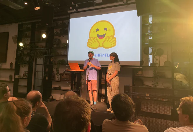
Hugging Face is a company that makes models and datasets freely available to the public in one place. Its website is very useful and is considered a standard in the field, and I wanted to wrap up this article by building a dataset in its format. A few months ago, I attended their meetup in Israel, and it was really nice to meet them face-to-face.
Step One: Combining Tables #
After processing the Llama-2 records, we’ll combine them with the records from the other models.
source_responses = pd.concat(
    [other_responses, llama_cleaned],
    axis=0
).reset_index(drop=True)
source_responses.head()
| response | sentiment | index |
|---|---|---|
Despite feeling tired, I’m energized by our team’s progress and the difference we’re making. | positive | 0 |
Despite the pain of loss carving deep, it etches into me the lessons of love and resilience. | negative | 1 |
“In this fleeting moment, I am deeply touched by the beauty around me and filled with gratitude." | positive | 2 |
“Despite the latest news being as dull as dishwater, I find solace in the simple joys of life." | negative | 3 |
“As the leaves fell whispering the inevitable change, I braced for the cold with a warm heart." | negative | 4 |
Step Two: Renaming Columns and Shuffling #
First of all, it was important to me to shuffle the df so there would be no chance of the records being ordered in a way that could affect the model during training. Also, to make sure model training goes smoothly without configuration issues, we’ll change the labels to numbers rather than text and rename the columns.
from datasets import Dataset, DatasetDict
import pandas as pd

# Shuffle the dataframe
shuffled_responses = source_responses.sample(frac=1).reset_index(drop=True)

# Map labels to numbers
label_mapping = {'positive': 1, 'negative': 0}
shuffled_responses['sentiment'] = shuffled_responses['sentiment'].map(label_mapping)
shuffled_responses = shuffled_responses.rename(columns={'response': 'text', 'sentiment': 'labels'})

shuffled_responses.head()
| text | labels | index |
|---|---|---|
As the seasons change, so does my energy level… | 1 | 0 |
Even though I’m exhausted from searching high … | 1 | 1 |
Despite the grueling work environment, where “… | 0 | 2 |
“Every cloud has a silver lining, for even our… | 1 | 3 |
Despite the setbacks and challenges of loss, m… | 0 | 4 |
Step Three: Creating a Dataset #
We’ll create features to map what the numbers we used as labels represent. We’ll also split the dataset into training and test sets. Separating training and test data is important so we can evaluate the model’s results using data it has never seen before. Then, using the DatasetDict function, we can create our dataset.
from datasets import Dataset, DatasetDict, Features, ClassLabel, Value

# Define dataset features, including label descriptions
features = Features({
    'text': Value('string'),
    'labels': ClassLabel(names=['negative', 'positive'])
})

# Split the shuffled dataframe (90% for training, 10% for testing)
threshold = 0.9
split_index = int(threshold * len(shuffled_responses))
df_train = shuffled_responses[:split_index]
df_test = shuffled_responses[split_index:]

# Convert to Dataset with defined features
train_dataset = Dataset.from_pandas(df_train, features=features)
test_dataset = Dataset.from_pandas(df_test, features=features)

# Create DatasetDict
sentiments_dataset = DatasetDict({
    'train': train_dataset,
    'test': test_dataset
})

sentiments_dataset
DatasetDict({
    train: Dataset({
        features: ['text', 'labels'],
        num_rows: 900
    }),
    test: Dataset({
        features: ['text', 'labels'],
        num_rows: 99
    })
})
Summary #
We learned how to use natural language models to build a synthetic dataset so we can streamline various workflows. See you in the next article, where we’ll learn to train a BERT model using the dataset we learned to create 😀