Fine Tune DistilBERT

Transformers have taken language processing to new heights in a variety of ways. In this article, we’ll learn what Transformers actually are, what BERT is, and how they relate to LLMs. Then, using the synthetic dataset we created in the previous article, we’ll fine-tune a DistilBERT model.

Transformers #

How do they work? Why do they outperform Recurrent Neural Networks (known as RNNs), Gated Recurrent Units (known as GRUs), and Long Short-Term Memory networks (known as LSTMs) on sequence problems? What did I just say, anyway?

Attention is All You Need #

The 2017 paper “Attention is All You Need” brought an innovation to the field, introducing a new neural network called “Transformers.” The structure of Transformers is based on an encoding (encode) and decoding (decode) architecture that uses Attention.

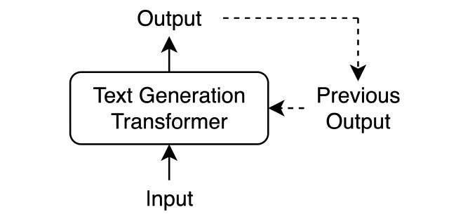
To understand the basic principles of the Attention mechanism, let’s look at an example of a generative model writing a dramatic story. First, the model receives input, processes it, and produces output. Then, we feed the original input back in along with the previous output, allowing the model to generate more output. This process lets the model build a dramatic story based on the initial input while taking the developing plot into account.

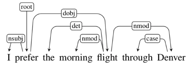
When the model generates text, it does so word by word. For each word it generates, it can refer back to (Reference) related words that came before it. During training, particularly in the ‘Backpropagation’ stage, the model learns to understand the relationships between words, allowing it to generate text in the right Context.

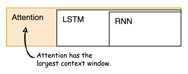
Unlike other models for Sequence Problems, the Attention-based mechanism does not run into short-term memory limitations. It can generate text while preserving long-range relationships by taking the ongoing flow of the text into account.

What does this mean in practice? Text enters the model as an “input sequence”—data fed in a particular order, where that order matters for processing. The model’s encoder translates this sequence into an abstract representation that stores all the information the model has gathered from the input. Then, the decoder takes this abstract representation and works to generate the output step by step. During this process, the decoder considers both the input and previously generated outputs. This allows the model to respond accurately to the original input.

Let’s take it apart and put it back together.

Input Embedding #

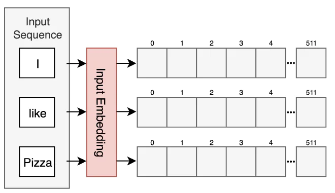
Each word in the sentence (input sequence) is translated into a vector of continuous values (a word embedding) that represents the word in space. These vectors are predefined in a dictionary and have 512 dimensions. The main idea behind each vector is that words with similar semantic meanings have similar representations in space. For more on this topic, see the Word2Vec article I wrote. After the Input Embedding layer generates a vector for each word in the sentence, we move on to the next layer, Positional Encoding.

Positional Encoding #

We now have a collection of vectors, each representing a word. The problem is that we aren’t accounting for which word comes before another. To address this, before feeding the vectors into the Encoder, we add information about each vector’s relative position in the sentence. Before we continue, why does this matter?

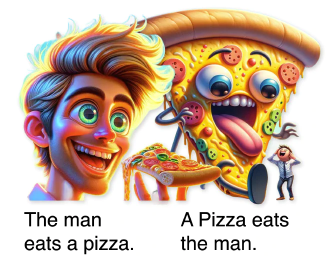
As you can clearly see, the positions of the words directly affect the meaning of the sentence.

To encode the position of each and every word, we need to find a method that meets the following criteria:

1. Unique encoding for each time-step - Each position in the sequence needs a distinct positional representation, allowing the model to distinguish between different positions in the sentence.
2. Consistent distance between any two time-steps - The model needs to be able to consistently identify the distance between two positions in the sequence. Typically, this means that the positional encoding should change gradually as we move from one position to another.
3. Should generalize to longer sentences - The encoding system needs to work with sentences of different lengths. It should not be limited to fixed-length sentences and should ideally support sentences longer than those seen during training.
4. Deterministic - The process of generating positional encodings must be deterministic: a given position should always produce the same encoding. This consistency is essential for the model to reliably learn positional dependencies.

The researchers discovered that sine and cosine functions could be used to create a unique encoding for each word in a sentence while accounting for the conditions we discussed above. These functions generate vectors with the same length as the input embedding. In the illustration below, each row is the vector we’ll add to the vector representing a word, and each column represents a different dimension (I reduced this to 100 dimensions for illustration). The resulting pattern looks like zebra stripes, with even positions using sine and odd positions using cosine. This is an efficient method that helps the model identify each word’s position.

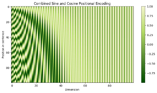
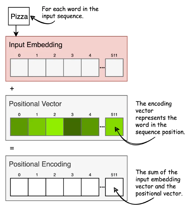
We’ll add the vectors to their corresponding Input Embeddings. This lets the model know the vectors’ relative positions and derive meaning from them. Sine and cosine functions were chosen together because they have linear properties—much like the ordering of the individual words. More on this topic. After this layer, the input is called the “Input Sequence.”

Encoder Layer #

The Encoder layer processes the Input Sequence to extract important information, so that the model can ultimately understand the input’s meaning and generate appropriate output. This layer has several components, each with a specific purpose.

Self-Attention #

The Self-Attention mechanism allows inputs to see one another (“self”) and determine which ones deserve more focus (“attention”). The output is this comparison, with scores for each word relative to another word in the sentence.

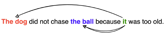
In the sentence below, does the word “it” refer to the street or the animal? It’s obvious to us that a street can’t be tired, but this is harder for the model. Self-Attention is a mechanism that lets a word express how relevant it is relative to every other word in the sentence, helping the model understand the relationships between the words and the meaning of the sentence as a whole.

Step 1: Preparing Inputs #

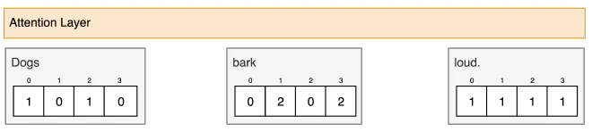
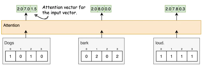
We’ll start by creating a vector for each word in the sentence. For this demonstration, all vectors have 4 dimensions. Remember, we’ve already performed Positional Encoding, so each vector also has its position in the sentence embedded in it.

Step 2: Creating Weight Matrices #

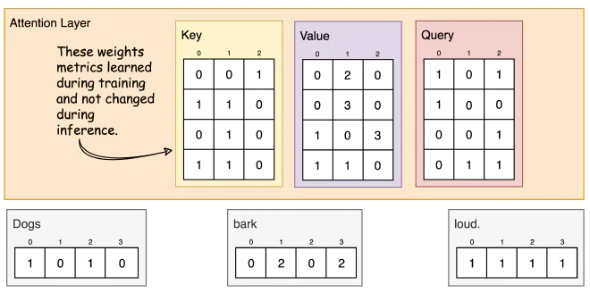
Projection matrices, learned during training, process the inputs from different perspectives. There are three types of projection matrices: “Query,” “Key,” and “Value.” In the paper, these matrices have 64 dimensions. I suggest remembering the colors to make the diagrams easier to follow.

Step 3: Multiplying the Matrices by the Inputs #

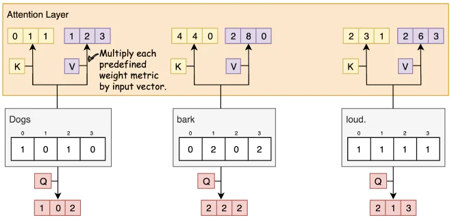
For each input, we’ll multiply its values by all the projection matrices. We’ll feed the results of the Key and Value matrices into the Attention layer and set the Query matrices aside.

An example of calculating the Key matrix for the word Dogs:

               [0, 0, 1]
[1, 0, 1, 0] x [1, 1, 0] = [0, 1, 1]
               [0, 1, 0]
               [1, 1, 0]

Step 4: Calculating the Attention Score #

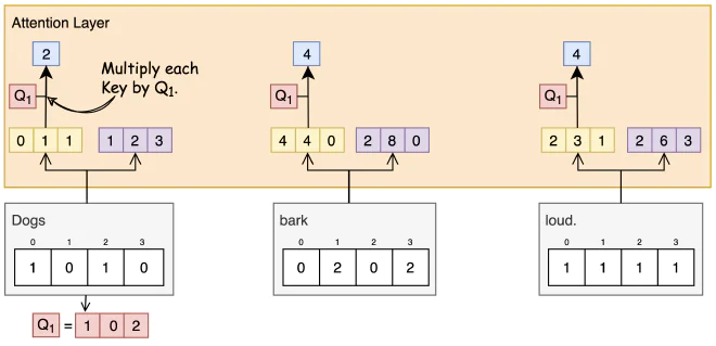
To calculate the Attention score for the first word (Dogs) relative to the rest of the sentence, we’ll multiply its Query, Q1 (red), by the Key vectors (yellow) for all the words in the sentence. This score lets us measure how other words relate to the word being processed—Dogs.

Step 5: Scaling & Softmax #

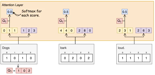
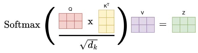
After calculating the score, we’ll divide the result by the square root of the Key dimension (for example, by 8 if there are 64 dimensions, as in the paper) to “soften” the correlation between Query and Key. Why? So we can control how much the model needs to change its weights during training (the size of the gradients) and prevent Vanishing gradients (skipping over the minimum error rather than approaching an optimal solution). For simplicity, I haven’t shown this in the diagram.

The scores are passed through the Softmax function to convert them into values with a fixed frequency, so that their values fall between 0 and 1.

Step 6: Multiplying Scores by Values #

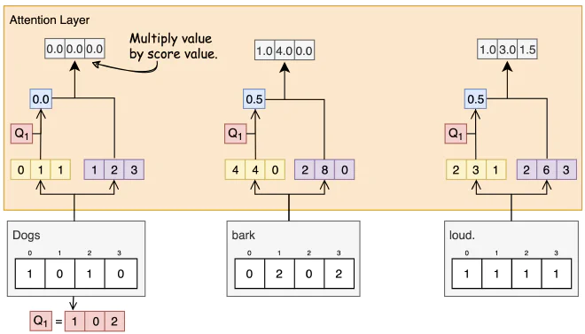
The score after Softmax (blue) is multiplied by its corresponding Value vector (purple).

Step 7: Summing the Weights #

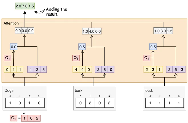
We’ll take all the vectors with each word’s weights and the multiplication results to obtain the output of the Attention layer: how much each word affects another word in the sentence. In our example, we only considered the first word, Dogs.

  [0.0, 0.0, 0.0]
+ [1.0, 4.0, 0.0]
+ [1.0, 3.0, 1.5]
-----------------
= [2.0, 7.0, 1.5]

The vector we obtained describes the relationship between the first word and all the other words in the sentence: “Dogs” affects itself by 2.0, the word “bark” by 7.0, and the last word, “loud,” by 1.5 (made-up numbers).

Step 8: Calculating Attention for the Remaining Words #

We’ll repeat the steps we followed to calculate Attention for the remaining words in the sentence.

Matrix Multiplication #

One of the main advantages of Self-Attention is that it allows vectors to be processed in parallel. Instead of performing these operations (calculating importance scores, Softmax, multiplying by Value, etc.) for each word and its comparison with every other word, one word at a time, we can perform them in parallel for all words in the sentence using matrix-matrix operations.

In practice, when we perform Self-Attention, we prepare three matrices (Q, K, V) from the learned weights and the sentence’s vectors. Then, through matrix multiplication, we calculate all the relationships (Context) between every pair of words in the sentence in parallel.

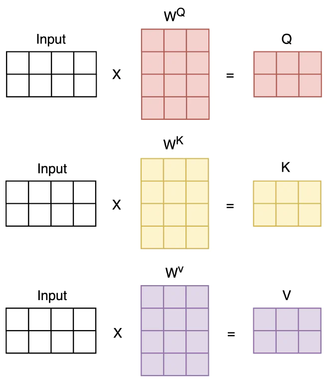
The calculation is identical, except that this time we have matrices instead of vectors.

Multi-Head Attention #

Rather than limiting the model’s perspective to a single Attention layer, the researchers discovered that different projection matrices for queries, keys, and values could be defined, with each set of three assigned its own Attention head and learned separately. This means that instead of a single Attention layer focusing on one context for each sentence, we can examine a broader range of contexts in parallel, allowing the model to learn more complex relationships between words from several different angles. In the paper, the researchers defined 8 “heads” for the Attention layer.

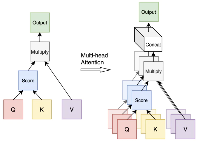
During Multi-Head Attention, each “head” independently computes Queries, Keys, and Values. This lets each head focus on a distinct subset of information from the overall data. In this process:

1. Each head applies an Attention function to the Queries, Keys, and Values using different pretrained weights, producing an output vector unique to that head.
2. Once all the heads have finished their calculations, the model combines their outputs into a single expanded vector by concatenating the output vectors side by side, bringing the information from all the heads into one structure.
3. The final step involves multiplying the combined vector by another projection matrix, which also has its own unique weights. The goal is to convert the combined vector to the dimensions required by the model’s next layers and integrate what all the Attention heads have learned, allowing data to keep flowing through the learning process.

Combining outputs from multiple heads in this way increases the model’s ability to capture and process a wide range of perspectives and details, improving its performance in understanding text.

Add & Norm #

The Attention layer is followed by an Add and Norm layer. Here, we add the Input Embedding to the vector produced at the end of the Attention layer. This technique is known as a “Residual Connection,” and its purpose is to combine the contextual knowledge learned in the Attention layer with the original input. This lets us carry the original input through deeper layers of the model and, once again, avoid Vanishing gradients.

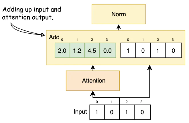
After adding the vectors, the summed vector passes through the Norm layer (short for Normalization). There are many normalization methods, with two main ones. Batch Norm calculates the mean and variance for each feature in a batch. For example, in a batch of words, Batch Norm calculates the mean and variance for each feature and normalizes each one using those statistics. This method helps stabilize learning but is less effective for sequential models such as Transformers, where the number of words per sentence varies.

Layer Normalization, on the other hand, calculates the mean and variance across all features for each sentence. Each sentence is normalized using the statistics of all its features. This method is particularly suitable for sequential models and has proven useful in NLP tasks. The Transformer architecture uses Layer Normalization because it does not depend on batch size and handles sequential data efficiently.

Why has this layer proven useful and been adopted in a variety of other language and deep learning models?

1. Faster Training - Changes the scale of the values, reducing model training time.
2. Bias - Prevents the model from leaning toward extreme values.
3. Weights Explosion - Keeps the model’s weights within a fixed range.

Feed Forward #

The Attention layer has distilled the relationships between words in the sentence. The next layer, Feed Forward, processes these contexts for each word separately, adding the ability to examine the relationships between words more deeply and produce a nonlinear representation of the sentence. This layer is also called a fully connected feed-forward network (FFN). It processes each word in the sentence separately and, with a GPU, processes them in parallel.

The FFN consists of two Dense layers, with ReLU as the activation function between them. ReLU allows the model to process data nonlinearly and learn complex patterns—which is exactly the purpose of this layer. Its output has the same dimensions as the words we feed into it (d_model=512).

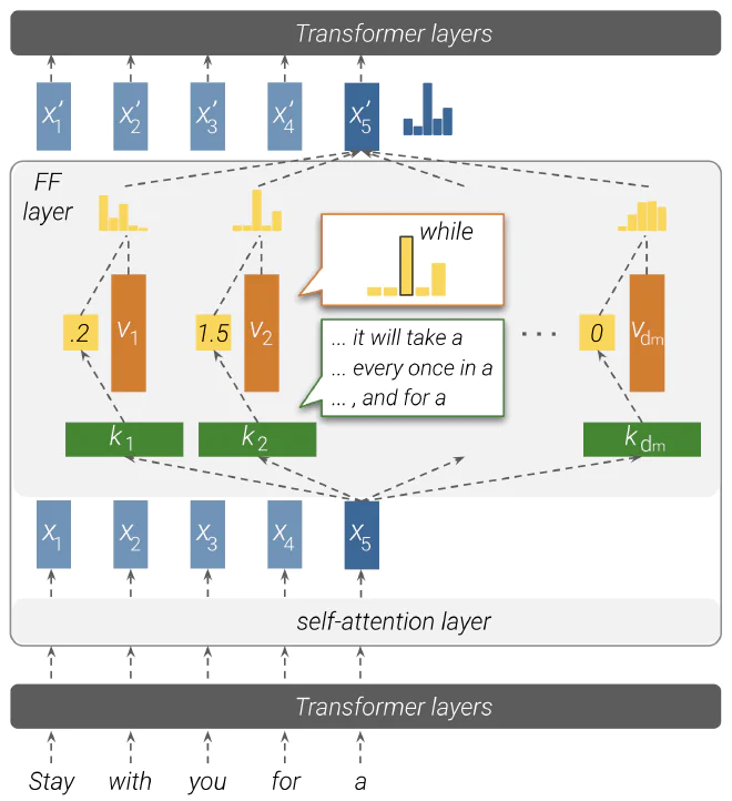
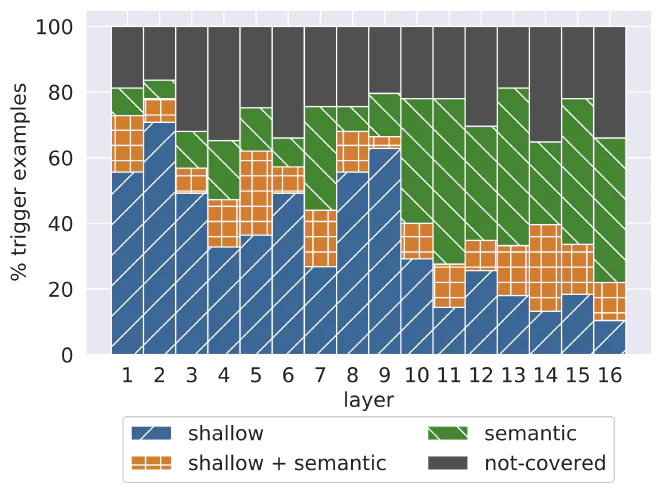
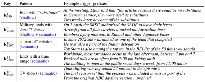
The paper “Transformer Feed-Forward Layers Are Key-Value Memories” notes that FFN layers play a central role in detecting key patterns in text. As the graph shows, the lower layers detect shallow patterns, such as syntactic elements, while higher layers reach deeper semantic patterns in sentences.

Examples of sentences by layer (the number above K represents the layer’s depth):

Add & Norm #

After the Feed Forward layer, we have another Add & Norm layer, just as we did after the Multi-Head Attention layer.

Transformer Summary #

We discussed the unique structure of the Encoder block within a Transformer model, went through each layer, and learned how it works. Although we also touched on the Decoder block, it’s important to remember that, for this discussion—especially when it comes to BERT—its role isn’t really relevant. We focused on the parts that truly matter for understanding the building blocks of Transformer models, particularly the Attention layers that extract and analyze the relationships and dependencies between words in a sentence.

BERT #

BERT is a model that changed the game in natural language processing and preceded large language models (LLMs). At its core, it is based on an Encoder component. This means the model focuses on learning and understanding text without getting into further technical details. BERT has a wide and varied range of real-world applications, from text comprehension and machine translation to automatically generating answers to questions.

BERT Model Structure #

Our goal is to distinguish between different classes based on sentences. Let’s take apart and rebuild a simplified BERT model.

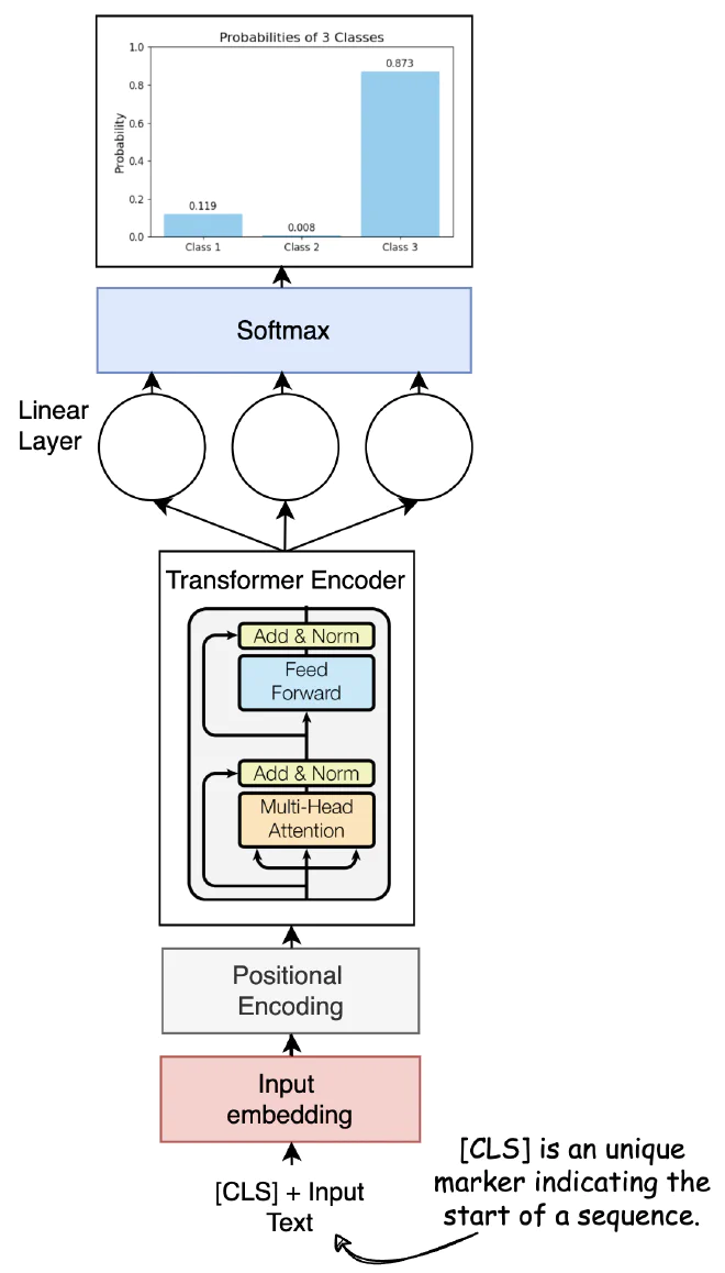
• Input Text - The initial text we need to classify.
• Tokenizer - Processes the input text, splitting it into tokens that BERT can understand.
• Adding the [CLS] Token - Adds [CLS] at the beginning of the input. This token aggregates the input’s representation for the classification we’ll perform later.
• Embedding Layer - Maps each token to a single vector.
• Transformer Encoder - The heart of BERT, which we discussed in the first part of the article. The embedded vector passes through several layers of self-attention and feed-forward networks to produce embeddings with relationships and dependencies between words in the sentence. For simplicity, we’ll treat this as a single unit.
• Output [CLS] Token - Extracts the final embedding of the [CLS] token from the Transformer encoder’s output.
• Linear Layer - A fully connected layer that projects the [CLS] token’s embedding into a vector whose length equals the number of classes in the classification task.
• Softmax - The softmax function produces a normal distribution over the classes.
• Predicted Class - The final prediction: the class with the highest probability of matching the sentence. Each class has a score.

DistilBERT #

To make our work easier and faster, we’re using a smaller version of the model, DistilBERT, which offers good performance while requiring fewer resources and running much faster.

The paper DistilBERT, a distilled version of BERT states:

A Quick Reminder #

Now that we’ve created a Synthetic Dataset using LLMs, we’ll use it to fine-tune a DistilBERT model. As a reminder, we have sentiments_dataset, a DatasetDict object from the datasets library:

# Create DatasetDict
sentiments_dataset = DatasetDict({
    'train': train_dataset,
    'test': test_dataset
})

sentiments_dataset

DatasetDict({
    train: Dataset({
        features: ['text', 'labels'],
        num_rows: 900
    }),
    test: Dataset({
        features: ['text', 'labels'],
        num_rows: 99
    })
})

Let’s take a random look at a few records in the training set:

# For the training set
train_sample = sentiments_dataset['train'].select(range(5))
print("Training Set First 5 Rows:")
for i in range(5):
    print(train_sample[i])

{'text': '"Despite the recent events, making new friends [...]"', 'label': 0}
{'text': "Despite the weariness from past hurdles and the [...]", 'label': 0}
{'text': '"Discovering a new interest in shopping immediat[...]"', 'label': 1}
{'text': 'Despite the long-term grind and competitive pres[...]', 'label': 0}
{'text': '"The autumn leaves falling gently onto my face [...]"', 'label': 1}

To give our environment access to Sagemaker and S3 resources, we’ll make sure AWS permissions are configured in the environment. It’s important to store the keys in an env file. Otherwise, we won’t be able to access these resources.

import os
import boto3
from dotenv import load_dotenv
import sagemaker

# Load environment variables from .env file
load_dotenv()

# Use the loaded environment variables to configure AWS access
aws_access_key_id = os.getenv('AWS_ACCESS_KEY_ID')
aws_secret_access_key = os.getenv('AWS_SECRET_ACCESS_KEY')
aws_default_region = os.getenv('AWS_DEFAULT_REGION')

# Initialize a boto3 session
boto3_session = boto3.Session(
    aws_access_key_id=aws_access_key_id,
    aws_secret_access_key=aws_secret_access_key,
    region_name=aws_default_region
)

Preprocessing #

When we explored the structure of Transformers, we learned that the Input Embedding layer translates text into a vector representation. That’s exactly the process we’re performing here. We use a tokenizer called distilbert-base-uncased, which maps the words in the dataset’s sentences to their vector representations. If a particular word appears multiple times, we may have to deal with redundant information. So we keep only the word’s ID as a reference to the predefined vocabulary.

The sentences in our dataset are not all the same length, and BERT requires equal-length inputs for its Input Embedding layer. To address this, we add an instruction to the tokenize function to apply padding using the padding='max_length' parameter. We’ll look at the longest text in the dataset and add the special [PAD] token to shorter texts. This token is designed to extend the vector without adding semantic meaning.

from datasets import load_dataset
from transformers import AutoTokenizer

# tokenizer used in preprocessing
tokenizer_name = 'distilbert-base-uncased'

# download tokenizer
tokenizer = AutoTokenizer.from_pretrained(tokenizer_name)

# tokenizer helper function
def tokenize(batch):
    return tokenizer(batch['text'], padding='max_length', truncation=True)

# Get train and test from sentiments_dataset
train_dataset = sentiments_dataset['train']
test_dataset = sentiments_dataset['test']

# tokenize dataset
train_dataset = train_dataset.map(tokenize, batched=True)
test_dataset = test_dataset.map(tokenize, batched=True)

The next step is to convert the dataset’s format to ’torch’ with the columns input_ids, attention_mask, and labels. We’ll be using the PyTorch library during training, and the format conversion also allows us to load and process the dataset efficiently. We’ll use a simple count to make sure we haven’t lost any records along the way.

# set format for pytorch
train_dataset.set_format('torch', columns=['input_ids', 'attention_mask', 'labels'])
test_dataset.set_format('torch', columns=['input_ids', 'attention_mask', 'labels'])

print(f"The length of the train dataset is {len(train_dataset)} records.")
print(f"The length of the test dataset is {len(test_dataset)} records.")

The length of the train dataset is 899 records.
The length of the test dataset is 100 records.

Uploading the Dataset to S3 #

Now that we’ve processed the dataset, we’ll upload it to S3.

# s3 key prefix for the data
s3_prefix = 'samples/datasets/sentiments_dataset'

# save train_dataset to s3
training_input_path = f's3://{sess.default_bucket()}/{s3_prefix}/train'
train_dataset.save_to_disk(training_input_path)

# save test_dataset to s3
test_input_path = f's3://{sess.default_bucket()}/{s3_prefix}/test'
test_dataset.save_to_disk(test_input_path)

Training the Model in Sagemaker #

This is actually my first time using AWS’s Sagemaker service. It’s an end-to-end managed environment: all we need to do is load the model, and everything is handled automatically. The first thing we’ll define is the model’s hyperparameters. In practice, the only parameter I played with was epochs, which specifies how many times the model goes through the training dataset. Since this is a small dataset, I set it to go through it 8 times.

from sagemaker.huggingface import HuggingFace

# hyperparameters, which are passed into the training job
hyperparameters = {
    'epochs': 8, # Changed it from 1 into 5
    'train_batch_size': 32,
    'model_name':'distilbert-base-uncased'
}

Next, we’ll define huggingface_estimator, which essentially contains all the instructions for training the model. The ’train.py’ file refines these settings further, but we won’t go into it in this tutorial. We used an ml.p3.2xlarge instance with 8 vCPUs and 61 GB of memory. It costs $3.80 per hour. Finally, we’ll specify the versions of the various libraries.

huggingface_estimator = HuggingFace(
    entry_point='train.py',
    source_dir='./scripts',
    instance_type='ml.p3.2xlarge',
    instance_count=1,
    role=role,
    transformers_version='4.26',
    pytorch_version='1.13',
    py_version='py39',
    hyperparameters = hyperparameters
)

The fit function starts the training process, referencing the dataset’s locations in S3. Note that we’ll receive plenty of logs, some of which will be useful later for understanding the model’s performance.

# starting the train job with our uploaded datasets as input
huggingface_estimator.fit({'train': training_input_path, 'test': test_input_path})

2024-03-12 19:55:54,252 loaded train_dataset length is: 899
2024-03-12 19:55:54,252 loaded test_dataset length is: 100
[...]
2024-03-12 19:58:17,831 Waiting for the process to finish and give a return code.
2024-03-12 19:58:17,831 Done waiting for a return code. Received 0 from exiting process.
2024-03-12 19:58:17,832 Reporting training SUCCESS

Since this is an expensive instance, let’s make sure it isn’t still running:

sagemaker_session = sagemaker.Session()
sagemaker_client = sagemaker_session.sagemaker_client
job_name = huggingface_estimator.latest_training_job.name
response = sagemaker_client.describe_training_job(TrainingJobName=job_name)
print(response['TrainingJobStatus'])

Completed

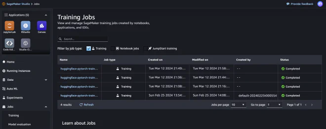
We can also verify this through the Sagemaker website. If the instance is marked “Completed,” it means we’re no longer being charged for it.

Training result #

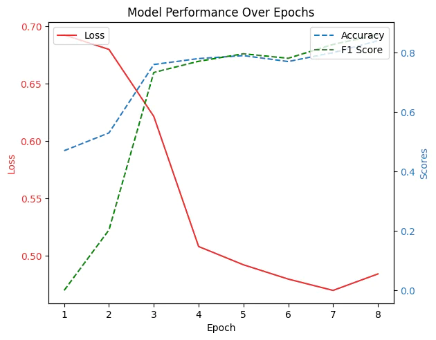
Based on the logs we received during training, we can draw some insights into the model’s training and quality:

Loss - Around the third epoch, the loss drops significantly, suggesting that the model learns quickly in its early stages. Toward the eighth epoch, we can see a small jump, suggesting the onset of overfitting.

Accuracy and F1 Score - Both metrics rise as training progresses, which is a good sign that the model is getting better and better at its assigned task. The F1 Score, a more complex metric that balances Precision and Recall, shows a similar trend to Accuracy, indicating an overall improvement rather than simply better classification of one category at the expense of the other.

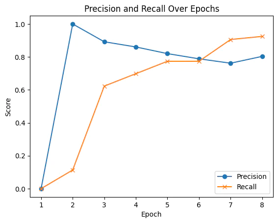
Precision and Recall - Precision starts very high and then stabilizes, while Recall rises consistently until the seventh epoch before dipping slightly. What does this mean in practice? Precision is a measure of how many results our model labeled as positive (for example, positive reviews) are actually positive. Recall is a measure of how many of the positive examples that really exist in our data the model found.

In the graph, the model started with very high precision—suggesting that all the results it classified as positive were correct. After that, Precision didn’t change much, but Recall continued to rise, meaning the model began finding more and more of the actual positive examples in the data. That’s good, because it means the model wasn’t just avoiding mistakes; it was also getting better at identifying what it needed to identify.

In the final epoch, Recall dipped slightly—meaning the model may have missed a few examples or made more mistakes in identifying positive results. This also looks like an indication of overfitting: the model memorized the dataset and won’t perform as well when we use it on data it hasn’t seen.

Deploying the endpoint #

Now that we’ve trained the model, we want to deploy it to an endpoint so we can use it outside our Python notebook. We’ll use the deploy() function to deploy it to an instance.

predictor = huggingface_estimator.deploy(1, "ml.g4dn.xlarge")

A demonstration of using the live model:

sentiment_input= {"inputs":"worst day ever"}
predictor.predict(sentiment_input)

Let’s delete the endpoint. Why? Because it stays running all the time, regardless of usage.

predictor.delete_model()
predictor.delete_endpoint()

Deploy Serverless Endpoint #

How can we deploy an endpoint that runs according to demand? A Serverless Endpoint is the answer. The endpoint will remain online, waiting for an initial message from the client. After a cold start, which involves actually loading the model into the endpoint (and a delay of a few seconds), the endpoint will be available as though it were hosted on a server running 24/7.

To deploy a HuggingFace model to a Serverless Endpoint in Sagemaker, we’ll follow these steps:

1. huggingface_model - Define the model. We’ll access S3 to retrieve the model and its tokenizer.
2. serverless_config - Configure the endpoint. I allocated 6 GB of memory and allowed 16 concurrent executions.
3. deploy - Bring the Serverless Endpoint online.

import sagemaker
from sagemaker.huggingface import HuggingFaceModel
from sagemaker.serverless import ServerlessInferenceConfig
from sagemaker.huggingface.model import HuggingFaceModel

# Specify the S3 URI of the model.tar.gz file
model_data = 's3://sagemaker-us-east-1-XXXXXXXXXXXXX/huggingface-pytorch-training-2024-03-12-19-49-02-465/output/model.tar.gz'
role = 'arn:aws:iam::XXXXXXXXXXXXX:role/service-role/AmazonSageMaker-ExecutionRole-20240225T000555'

# Create the HuggingFaceModel object
huggingface_model = HuggingFaceModel(
    model_data=model_data,
    role=role,
    transformers_version='4.6.1',  # Specify the appropriate version
    pytorch_version='1.7.1',       # Specify the appropriate version
    py_version='py36',             # Specify the appropriate Python version
)

# Specify the serverless inference configuration
serverless_config = ServerlessInferenceConfig(
    memory_size_in_mb=6144,  # Adjust based on your model size
    max_concurrency=16,      # Set the maximum concurrency for your endpoint
)

# Deploy the model as a serverless endpoint
predictor = huggingface_model.deploy(serverless_inference_config=serverless_config)

# Now you can use the `predictor` object to make predictions

---!

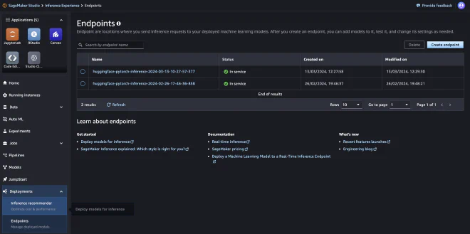
In the screenshot, you can see two live Serverless Endpoints in the Sagemaker interface:

Let’s test the Serverless Endpoint with an example:

input = """"
'I rented I AM CURIOUS-YELLOW from my video store because of all the controversy that surrounded it when it was first released in 1967. I also heard that at first it was seized by U.S. customs if it ever tried to enter this country, therefore being a fan of films considered "controversial" I really had to see this for myself.<br /><br />The plot is centered around a young Swedish drama student named Lena who wants to learn everything she can about life. In particular she wants to focus her attentions [...]'
""""
sentiment_input = {"inputs": input}
predictor.predict(sentiment_input)

[{'label': 'LABEL_0', 'score': 0.9690449237823486}]

Evaluate BERT on IMDB Dataset #

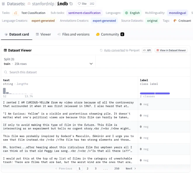
IMDB, in collaboration with Stanford, put together a dataset of moviegoers’ reviews. Each review is labeled as either negative or positive. I wanted to see whether a model trained on language model outputs would align with a dataset created by people.

Downloading the Dataset #

The first step is to load the dataset using the datasets library we used earlier.

from datasets import load_dataset

# dataset used
dataset_name = 'imdb'
dataset = load_dataset(dataset_name)
dataset

DatasetDict({
    train: Dataset({
        features: ['text', 'label'],
        num_rows: 25000
    })
    test: Dataset({
        features: ['text', 'label'],
        num_rows: 25000
    })
    unsupervised: Dataset({
        features: ['text', 'label'],
        num_rows: 50000
    })
})

We can see that the dataset contains 100,000 records, of which 50,000 are labeled.

Classifying 25,000 Records #

Once we’ve downloaded it, the next step is to go through it and see what the model predicts. The code that handles this is divided into three parts:

1. trunc_text - Shortens the text to the maximum number of tokens the model can accept. The maximum is 512, but I went with 450 to be on the safe side.
2. make_prediction - Uses the model to classify the text as negative or positive. This function returns a Dict containing the prediction, the expected prediction, and the confidence level.
3. ThreadPoolExecutor - A threaded process running 16 times in parallel, scanning the training data and checking what the model thinks each record is. The training set contains 25,000 records—did someone say large?

from transformers import AutoTokenizer
from concurrent.futures import ThreadPoolExecutor, as_completed
from tqdm import tqdm

tokenizer_name = 'distilbert-base-uncased'
tokenizer = AutoTokenizer.from_pretrained(tokenizer_name)

def trunc_text(text, max_length = 450):
    # Truncate the tokens to the maximum length (512 tokens)
    # Reserved space for special tokens like [CLS], [SEP]
    
    # Tokenize the text
    tokens = tokenizer.tokenize(text)
    truncated_tokens = tokens[:max_length]
    
    # Convert the truncated tokens back to a string
    truncated_text = tokenizer.convert_tokens_to_string(truncated_tokens)

    return(truncated_text)

# Function to make prediction and format result
def make_prediction(item):
    text = item['text']
    true_label = item['label']
    trunc_input = trunc_text(text)
    text_input = {"inputs": trunc_input}
    prediction_result = predictor.predict(text_input)[0]
    predicted_label = 0 if prediction_result['label'] == 'LABEL_0' else 1
    confidence = prediction_result['score']
    
    return {
        'text': text,
        'label': true_label,
        'prediction': predicted_label,
        'confidence': confidence
    }

# Initialize list to hold processed data
data = []

# Using ThreadPoolExecutor to run multiple predictions in parallel
with ThreadPoolExecutor(max_workers=16) as executor:
    # Setup future tasks
    future_to_item = {executor.submit(make_prediction, item): item for item in dataset['train']}
    
    # Process as they complete
    for future in tqdm(as_completed(future_to_item), total=len(dataset['train']), desc='Predicting'):
        result = future.result()
        data.append(result)

Predicting: 100%|████████████████| 
25000/25000 [21:03<00:00, 19.78it/s]

After waiting 21 minutes, we successfully finished classifying the records.

Evaluation Results #

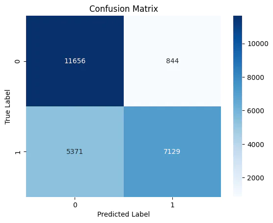
Confusion Matrix - A quick look shows that the model does make a large number of correct predictions: true positives and true negatives. However, it also has quite a few false positives, which may indicate that the model leans toward the negative and hasn’t reached the depth of understanding we expected.

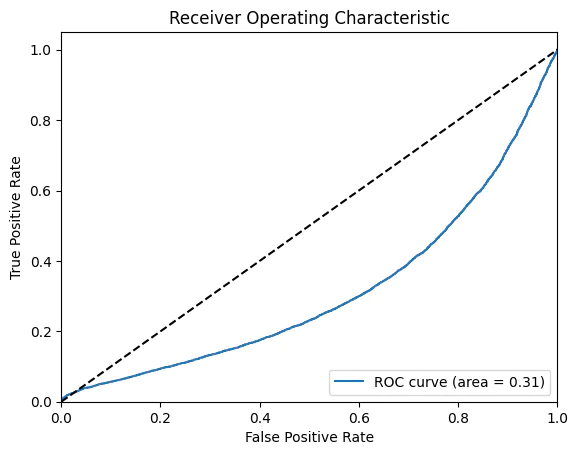
ROC - In this type of graph, an AUC below 0.5 means we’d be better off rolling a die than using the model, or using the opposite of its result. We can clearly see that there’s a problem here.

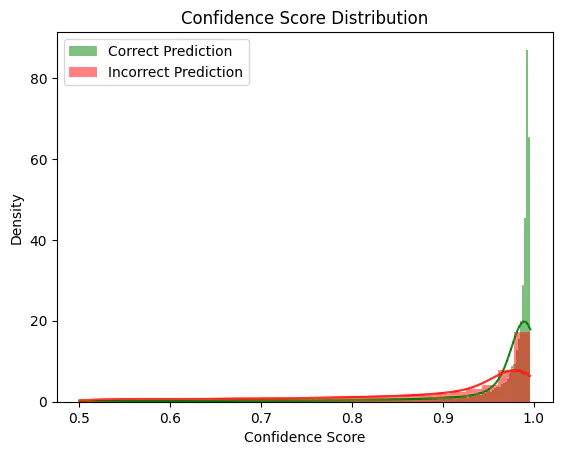
Confidence - Part of the model’s problem is its confidence in its text classifications. We can see a relationship between its confidence level and how often it is actually correct. We can also see that quite a few records fall between 0.5 and 0.9.

Covariate Shift #

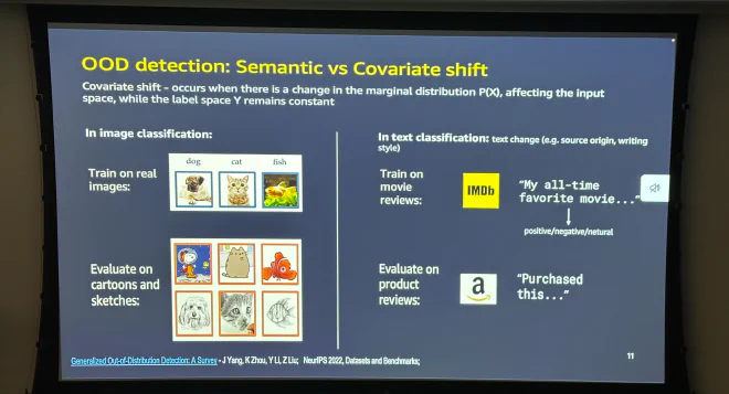
As fate would have it, while writing this article I attended a meetup at AWS (link to the recording). The first speaker discussed the problems with training a classification model on IMDB and testing it on Amazon. Small world, because that’s exactly what I did, only on steroids.

Conclusions #

If you’ve made it this far, first of all, thank you!

Now, seriously. This is a challenge we’ve shown to be possible, but not with the current implementation. My top 5:

1. Prompt - After creating the dataset, I noticed that all the generated sentences followed a cause-and-effect pattern. A very, very fixed structure, neither random nor varied. Although the topics and perspectives of the sentences written by the language models differed, the fact that the models did exactly what I asked actually hurt the model’s quality. Going forward, I would classify IMDB into categories and add few-shot examples to the prompt. Then I’d think about other ways to generate random records rather than follow templates.
2. Hyperparameter Tuning - It’s clear that more work is needed to optimize the model’s training process. We may have too few records, and at some point the model started memorizing the dataset.
3. Evaluation Dataset - Comparing a model trained on an LLM-based dataset with a human-made dataset is very challenging.
4. Confidence - We need to dig deeper into the model’s confidence. What types of records does it struggle to classify? Why?
5. Humans - As fun as this sounds, the human element is hard to copy and imitate, even with the most advanced language models on the market. In my opinion, the proof of concept is there, but quite a bit more work is needed.