Image Recognition with CNNs 📸
Sight is a sense we use from the moment we wake up until the moment we go to sleep. We cook, drive, recognize other people’s emotions, go about our daily routines, and perform countless other actions subconsciously.
When researchers began training networks to recognize faces, they managed to teach computers the features of human faces, allowing them to distinguish between faces, facial features, emotions, and more. This deep neural network (Deep Learning) consists of two parts. It turned out that we could replace the second part to handle unrelated tasks (for example, detecting a disease in an image of a body part) by retraining only that second part. Let’s dive in and learn together.
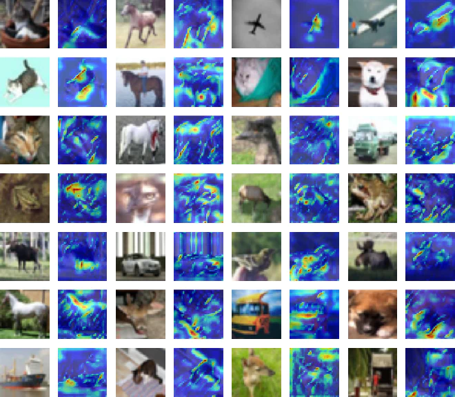
Do you see the image above? Interesting, right? We’ll learn what it represents and how to build something like it ourselves.
Convolutional Neural Networks #
Feeding an Image into the Model #
To a computer, an image is just pixels. As an example, I took a picture of the 16th president of the United States, Abraham Lincoln, and processed it in Python. We reduced the image’s dimensions and converted its pixels to grayscale so that each pixel would contain a single value between 0 and 255. The result is a two-dimensional matrix of numbers that represent the image.
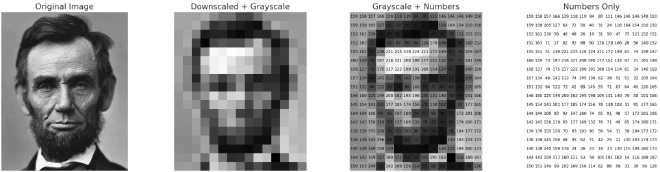
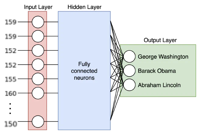
In the post Word2Vec for Beginners, we learned about the structure of neural networks. We could convert the matrix into an array and feed that array into a neural network’s input layer, seemingly solving the problem. Well, it turns out that isn’t quite enough: when we move from a two-dimensional image to a one-dimensional array, we lose the ability to make sense of spatial relationships, and image processing tasks such as face recognition would no longer be possible. In addition, if each pixel had its own dedicated neuron connected to every neuron in the hidden layer, we would end up with large, computationally heavy models, both to train and to run.
An Overview of a CNN Model #
Now that we understand why a solution based on our current knowledge doesn’t fit the task we want to solve, let’s learn about CNNs, short for Convolutional Neural Networks. To understand the model’s structure, the computation that gives it spatial vision, and the various terms involved, we’ll use a diagram of the VGG-16 image recognition model:
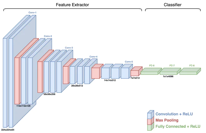
Feature Extractor (sometimes called the Backbone or Body): The part that sees the image. It is responsible for identifying various features: lines, corners, textures, and more. Several types of layers allow it to perform this feature extraction: convolution layers, pooling layers, and activation layers. This part maps and distills the important features in the image that will help the second part of the CNN.
Classifier (sometimes called the Head): Once the various features have been extracted, this part of the network handles the task we trained the model for, usually classifying whether an image contains an object or not. This part generally contains fully connected layers whose purpose is to predict the object appearing in the image.
Each layer has spatial dimensions (the X and Y axes) and a depth dimension (the depth of the layer). For example, the first layer is 224 by 224 with a depth of 64. As we progress through the model’s image processing, the spatial dimensions shrink while the depth dimension grows.
Let me put it simply: we have an image and a filter (usually a 3-by-3 matrix). We select a region of the image that is the same size as the filter. We perform a convolution operation between that region and the filter. We save the result and continue moving across the entire image. We can define an overlap between the regions. Once we have performed the same operation across the entire image, we pass the result through an activation function, giving the model the ability to represent relationships that are not just linear. This computation gives the model spatial vision. The model contains a sequence of Conv layers that perform the same computation and distill distinctive patterns. After that, we have fully connected layers that receive these patterns and perform the recognition task the model was trained for.
Now that we have a bird’s-eye view of how the model works, let’s learn how its components operate.
Part 1 - Feature Extractor #
To enable the model to identify features across the image and draw insights from them, we’ll use a method I like to call “tiling.” We select a specific region (patch) of the image for each neuron in the input layer. We slide the region in steps smaller than its length, so that the regions overlap. By dividing the image into regions like these, we preserve its spatial information and allow the model to extract distinctive features from it. The technical term for scanning these regions is “convolution.”
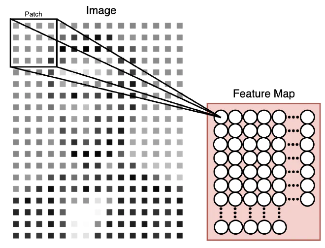
If you look closely, you’ll see that this is the same image of Lincoln from the beginning of the article. Unlike a fully connected neural network, here each neuron in the input layer has a patch of 4 pixels assigned to it. These pixels are spread across space, so the neuron is not limited to a one-dimensional view. But hold on, the illustration looks nice and the logic is clear, except for the most important detail: how do we actually calculate the value of each neuron?
Convolution Operation #
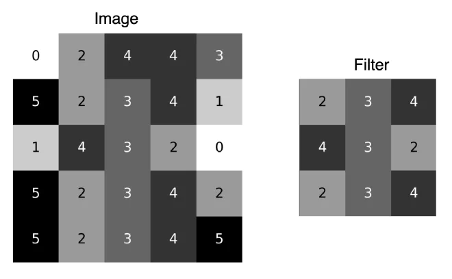
Meet the convolution operation, which we’ll use to extract distinctive patterns from images (these are the blue layers in the VGG-16 diagram). Let’s take an image and a 3-by-3-pixel filter as an example. What are the steps for computing a convolution?
- Patch: We define a patch that bounds the region of the image on which we want to perform a convolution. A patch has two main properties: its size and how many pixels it moves (stride) across the image at each step.
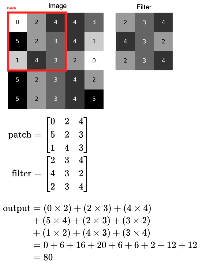
- Multiplication: For each patch in the image, we multiply each value by the value at the corresponding position in the filter. This multiplication is the building block of convolution.
- Summation: We sum the results of multiplying the 9 cells in the patch by the 9 cells in the filter.
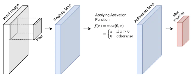
- Activation function: After multiplying and summing, we pass the new value through an activation function (as in the previous post). The commonly used activation function in CNNs is ReLU (Rectified Linear Unit). This function allows the model to learn complex patterns because it is nonlinear.
- Sliding: We slide across all the patches in the image to calculate the convolution value in every region.
- Collecting the results: After performing convolution across the entire image, we get an activation map, which we pass to additional layers in the model (if we hadn’t passed the values through an activation function, we would call the matrix a feature map). Sometimes we’ll want to add padding to avoid shrinking the image.
I drew an illustration to help you understand how the computation works at a high level:
MNIST Convolution Visualizer #
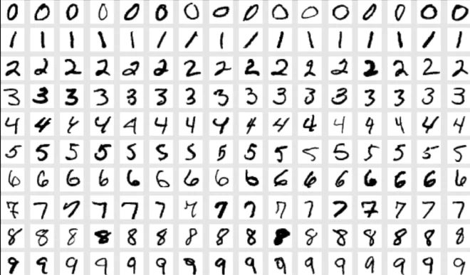
Before we continue, meet MNIST, a collection of images of handwritten digits, created in 1994. I developed a website that takes an image from the dataset, displays it, and performs a convolution operation. Before the CNN era, researchers discovered several useful filters for image processing. I took the popular ones and included them on the website, so users can choose which one to apply to the image. The website displays the values of the selected filter over the image, allowing users to explore and dig deeper. I’ve included a video so you can see the website in action.
| Filter Name | Explanation |
|---|---|
| Edge Detection | Edge detection identifies the outlines of objects in an image. The filter works by identifying sharp changes in color that correspond to edges. |
| Sharpen | A sharpening filter that increases the contrast between a pixel and its neighbors, emphasizing edges. |
| GaussianBlur | A blurring filter. Each pixel in the image is replaced by a weighted average of its neighboring pixels. The exact weights are defined by the filter. |
Pooling Layers #
In most CNN models, the layer size (spatial dimensions) typically shrinks as we go deeper into the model, as we can also see in VGG-16. The layer size is reduced using pooling layers (the red layers in the VGG-16 diagram), which come after several Conv layers. Although this may seem like a basic layer, a pooling layer significantly reduces the model’s computational footprint, helping avoid overfitting and reducing the model’s size, issues we want to avoid.
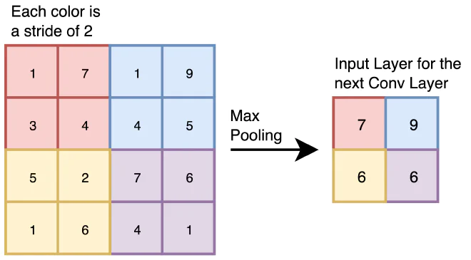
How does a pooling layer work? I’ll explain with an example. Let’s take a 4-by-4 image and divide it into 2-by-2 regions (stride). For each region, we’ll find the cell with the maximum value. There are two differences here compared with a convolution operator: the regions do not overlap, and the filter has no trained parameters, just a simple Max operation. After max pooling, the result passes to the next layer in the model.
Feature Extractor Summary #
Before moving on to the second part of the model, let’s summarize its first part, the feature extractor. We receive an input image, in our case 224 by 224. We perform a convolution operation using a filter. We place the results in a feature map, which we pass through an activation function to give the model the ability to represent nonlinear relationships. Then we reduce the size of the next layer through a max pooling layer. The resulting matrix is fed into the next Conv layer as input.
Part 2 - Classifier #
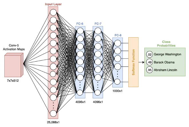
In VGG-16, the fifth and final Conv layer contains a 7-by-7-by-512 activation map (after max pooling). This layer contains various processed representations of the image that account for spatial relationships and many parameters the model identifies during training. Essentially, all that remains is to link these processed representations to the labels we want to identify, using a deep neural network.
Before the feature extractor’s output can enter the classifier, we need to flatten the matrix into a one-dimensional array, in our case of size 25,088, which will serve as the classifier’s input. It’s important to note that when we convert to a one-dimensional array, we still preserve the distinctive features the model extracted, so we don’t lose them along the way.
Once we have a one-dimensional array, we feed its values into a deep neural network with three layers. After the image passes through the model, we get numbers with no defined, bounded range. To turn these numbers into percentages, we normalize them using the Softmax function. The function takes the maximum and minimum numbers from the final layer (FC-8) and normalizes them to a range between 0 and 1, where 1 represents a 100% likelihood.
What happens with different images? Each image that goes through processing in the first part of the model will have a different activation map. Then, using the deep neural network, we can identify relationships between these maps and the labels. How? Every neuron contains a collection of weights whose values are adjusted during training to fit the different labels. What’s interesting is that we can’t really explain these relationships and the weights in the neurons, yet at the same time, we can use them to achieve the desired result.
Recognizing Objects in an Image #
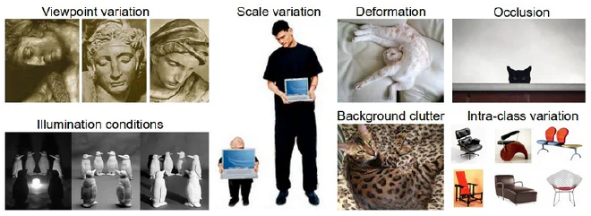
Although there are several types of tasks, we’ll focus on the main one, Classification, whose goal is to recognize objects in an image. If we want to train a model to recognize objects in images, it will need to extract distinctive features from the images in the dataset that point to patterns unique to each object, so it can tell them apart. As we all know, any object can be photographed in different ways: camera angle, amount of light, camera, and so on. Our model will extract the main features from the images, allowing it to distinguish between objects regardless of the variation in the images.
Implementing a CNN in Python #
Now that we’ve learned about the components of CNN models, their different layers, and the image processing operations they perform, it’s time to implement a model ourselves. We won’t implement a large model like VGG-16, but a smaller one that we can comfortably train on a personal computer.
Importing Libraries #
As we already know from previous tutorials, the first step before we start developing is to import the libraries we need.
As you can see, we’re using a library we haven’t worked with yet, called Tensorflow. This is an open-source library developed by Google. It allows us to download the image dataset, define the CNN model, and perform additional processing.
We’re also using the dataclass library. This library lets us store values in classes using a decorator. We’ll use this feature to create global variables to keep our code consistent and organized.
import os
import random
import numpy as np
import pandas as pd
import seaborn as sns
import matplotlib.pyplot as plt
from skimage.transform import resize

import tensorflow as tf
from tensorflow.keras import Sequential
from tensorflow.keras.layers import Dense, Conv2D, MaxPooling2D, Dropout, Flatten
from tensorflow.keras import models

from tensorflow.keras.datasets import cifar10
from tensorflow.keras.utils import to_categorical
from matplotlib.ticker import (MultipleLocator, FormatStrFormatter)
from dataclasses import dataclass
from typing import List
After importing the libraries, we’ll set a seed. What does that mean? To establish the neural network’s starting point, its weights are initialized randomly. A seed lets us fix the pseudorandom value, allowing us to generate random weights while also being able to reproduce them. This matters to us because when we train models, we want to make sure that the randomness of the network’s initial state before training does not affect the prediction results.
SEED_VALUE = 42

random.seed(SEED_VALUE)
np.random.seed(SEED_VALUE)
tf.random.set_seed(SEED_VALUE)
Loading the CIFAR-10 Dataset #
The CIFAR-10 dataset contains 60,000 images across 10 different classes. We can access it directly through Tensorflow using tensorflow.keras.datasets.
As you can see, we have a train/test split, allowing us to validate the model on data it did not see during training.
(X_train, y_train), (X_test, y_test) = cifar10.load_data()

print(X_train.shape)
print(X_test.shape)
(50000, 32, 32, 3)
(10000, 32, 32, 3)
Exploring the Dataset #
Before building the model and starting to train it, it’s important to take a look at the dataset. We’ll do this in two steps. Before we begin, the dataset’s classes are defined as indices from 0 to 9, so you’ll notice that I saved a separate variable, class_names, which we can use to map each index to its actual value.
Inspecting the Images #
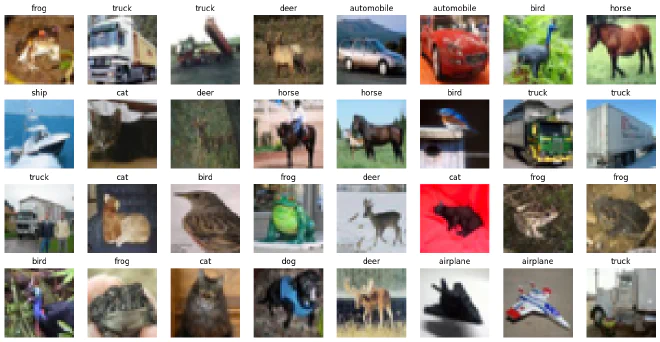
CIFAR-10 images are small, just 32 by 32 pixels. Some images will be hard even for us to make sense of.
plt.figure(figsize=(18, 9))

num_rows = 4
num_cols = 8

# Class names for CIFAR-10
class_names = ['airplane', 'automobile', 'bird', 'cat', 'deer',
               'dog', 'frog', 'horse', 'ship', 'truck']

for i in range(num_rows*num_cols):
    ax = plt.subplot(num_rows, num_cols, i + 1)
    plt.imshow(X_train[i,:,:])
    label_index = int(y_train[i])
    ax.set_title(class_names[label_index])
    plt.axis("off")
Checking Frequencies #
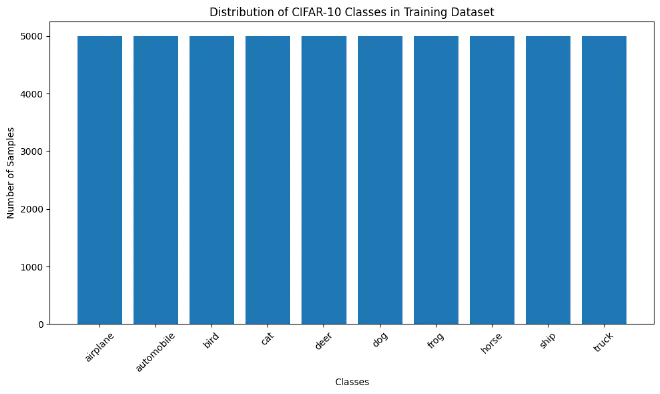
After taking a quick look at the images, it’s important to make sure the classes appear equally often and that no class has more examples than another. That situation would introduce bias into the model, which we want to avoid. We can see that the class frequencies are consistent, so we don’t need to worry about bias in the model.
# Count the occurrences of each label in the training dataset
unique, counts = np.unique(y_train, return_counts=True)

# Plot histogram
plt.figure(figsize=(10,6))
plt.bar(class_names, counts)
plt.xlabel('Classes')
plt.ylabel('Number of Samples')
plt.title('Distribution of CIFAR-10 Classes in Training Dataset')
plt.xticks(rotation=45)
plt.tight_layout()
plt.show()
Preparing the Dataset for Training #
Normalizing Colors #
A pixel contains three values: red, green, and blue (RGB), each between 1 and 255. We’ll need to normalize them so that they contain values between 0 and 1. We’ll do this by dividing the pixel by 255. For example, a pixel with a value of 128 will be converted to 0.502.
Normalization helps the neural network finish training faster and prevents it from getting stuck in a loop of local optima.
# Normalize images to the range [0, 1].
X_train = X_train.astype("float32") / 255
X_test  = X_test.astype("float32") / 255
Encoding #
One-hot encoding converts labels into a binary vector. Encoding ensures that the network doesn’t accidentally treat a category as a number whose order matters (ordinal data).
For example, suppose the labels ‘airplane’, ‘automobile’, and ‘bird’ in the dataset are represented as 0, 1, and 2, respectively. Without encoding, the model might think that ‘bird’ is actually twice ‘automobile’.
I took these three words as an example and showed how they would be encoded:
- ‘airplane ’ [1, 0, 0]
- ‘automobile ’ [0, 1, 0]
- ‘bird ’ [0, 0, 1]
# Change the labels from integer to categorical data.
print('Original (integer) label for the first training sample: ', y_train[0])

# Convert labels to one-hot encoding.
y_train = to_categorical(y_train)
y_test  = to_categorical(y_test)
print('After conversion to categorical one-hot encoded labels: ', y_train[0])
Original (integer) label for the first training sample:  [6]
After conversion to categorical one-hot encoded labels:  [0. 0. 0. 0. 0. 0. 1. 0. 0. 0.]
Configuration #
Before we implement and train the model, we have one last step. We’ll define the parameters in advance in one central place, so that if we want to adjust anything, we can do so without getting lost in the code.
Using dataclasses, we can create DatasetConfig, TrainingConfig, and CompileConfig as classes with parameters we’ll use during model training.
@dataclass(frozen=True)
class DatasetConfig:
    NUM_CLASSES:  int = 10
    IMG_HEIGHT:   int = 32
    IMG_WIDTH:    int = 32
    NUM_CHANNELS: int = 3

@dataclass(frozen=True)
class TrainingConfig:
    EPOCHS:        int = 31
    BATCH_SIZE:    int = 256
    LEARNING_RATE: float = 0.001
    SPLIT:         float = 0.3

@dataclass(frozen=True)
class CompileConfig:
    OPTIMIZER: str = 'rmsprop'
    LOSS: str = 'categorical_crossentropy'
    METRICS: List[str] = ('accuracy',)
Implementing the CNN Model #
We’ve reached the part we’ve been waiting for: defining a CNN model and training it on the CIRFAR-10 dataset. Here are the steps we’ll follow:
- Create a model using deep layers
- Compile the model
- Train the model using
model.fit()
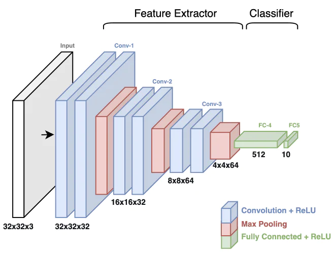
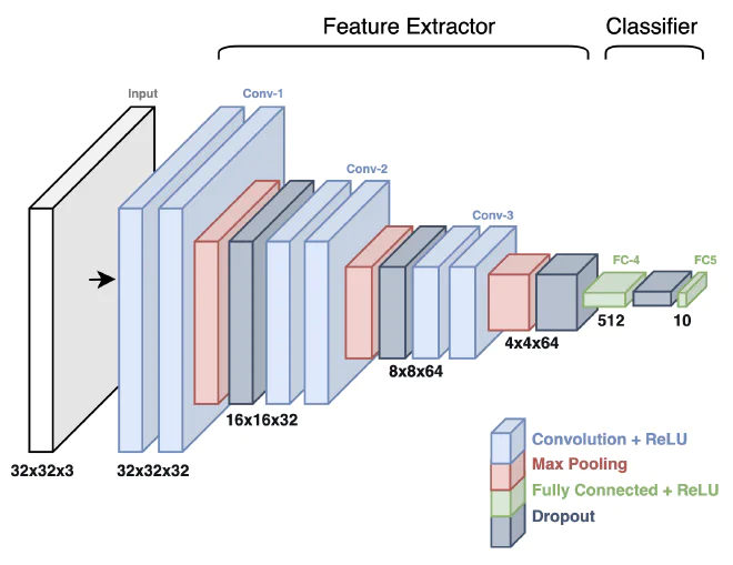
The structure of the CNN we’re building is inspired by VGG-16, which we discussed at the beginning of the article. However, our model has fewer layers and a significantly smaller input size, so we can train it locally without needing a more powerful computer. The model contains three Conv layers followed by two fully connected layers.
Notice that the input layer is 32x32x3, meaning a 32x32 image with 3 color channels (RGB), so our model takes all the colors into account rather than ignoring them.
Convolution Layers #
- In the first block, we have two Conv layers with 32 filters, paired with a max pooling layer.
- The second block is similar, but with 64 filters.
- The third block is identical to the second.
In all three Conv blocks, the filters will be 3x3. We’ll use same padding to keep the size constant, and the activation function will be ReLU.
Classifier Layers #
- We’ll use the
Flattenfunction to “flatten” the 4x4x64 activation matrices into a one-dimensional array of size 1024. - We’ll add a fully connected layer with 512 neurons and a ReLU activation function, as usual.
- Finally, an output layer with 10 neurons. We use 10 neurons because we have 10 types of objects (classes) the model needs to distinguish between.
As you know, all the numbers and sizes I’ve mentioned are hyperparameters that we can change and tune as we train the model more times and discover the best combination. However, we need to be careful not to overtrain the model and cause overfitting. I’ll note that we could also have created a dedicated dataclass here to reduce repetitive lines of code, but as part of the learning process, I chose to write out all the model’s layers to make it clearer what we’ve actually built.
def cnn_model(input_shape=(32, 32, 3)):
    model = Sequential()

    # ================================
    # Convolutional Blocks
    # ================================

    # ----- Conv Block 1: 32 Filters, MaxPool. -----
    model.add(Conv2D(filters=32, kernel_size=3, padding='same', activation='relu', input_shape=input_shape))
    model.add(Conv2D(filters=32, kernel_size=3, padding='same', activation='relu'))
    model.add(MaxPooling2D(pool_size=(2, 2)))

    # ----- Conv Block 2: 64 Filters, MaxPool. -----
    model.add(Conv2D(filters=64, kernel_size=3, padding='same', activation='relu'))
    model.add(Conv2D(filters=64, kernel_size=3, padding='same', activation='relu'))
    model.add(MaxPooling2D(pool_size=(2, 2)))

    # ----- Conv Block 3: 64 Filters, MaxPool. -----
    model.add(Conv2D(filters=64, kernel_size=3, padding='same', activation='relu'))
    model.add(Conv2D(filters=64, kernel_size=3, padding='same', activation='relu'))
    model.add(MaxPooling2D(pool_size=(2, 2)))

    # ================================
    # Classifier
    # ================================

    model.add(Flatten())
    model.add(Dense(512, activation='relu'))
    model.add(Dense(10, activation='softmax'))

    return model
Now that we’ve created a function that defines and returns a model, we can call it and display a summary. I suggest spending a few minutes trying to understand what we’re seeing here. Personally, I found the summary an interesting way to see our model implemented. What’s even more interesting is the number of parameters we’ll be training: 670 thousand, a lot, right?
model = cnn_model()
model.summary()
Model: "sequential"
_________________________________________________________________
Layer (type)                Output Shape              Param #
=================================================================
conv2d (Conv2D)             (None, 32, 32, 32)        896

conv2d_1 (Conv2D)           (None, 32, 32, 32)        9248

max_pooling2d (MaxPooling2  (None, 16, 16, 32)        0
D)

conv2d_2 (Conv2D)           (None, 16, 16, 64)        18496

conv2d_3 (Conv2D)           (None, 16, 16, 64)        36928

max_pooling2d_1 (MaxPoolin  (None, 8, 8, 64)          0
g2D)

conv2d_4 (Conv2D)           (None, 8, 8, 64)          36928

conv2d_5 (Conv2D)           (None, 8, 8, 64)          36928

max_pooling2d_2 (MaxPoolin  (None, 4, 4, 64)          0
g2D)

flatten (Flatten)           (None, 1024)              0

dense (Dense)               (None, 512)               524800

dense_1 (Dense)             (None, 10)                5130

=================================================================
Total params: 669354 (2.55 MB)
Trainable params: 669354 (2.55 MB)
Non-trainable params: 0 (0.00 Byte)
_________________________________________________________________
Compiling the Model #
After defining all the model’s layers and seeing what it looks like, we need to compile it. What does compiling involve?
Loss Function: How the model’s prediction is compared with the actual result. In our case, we’ll usecategorical_crossentropy, which is suitable for classification problems with one-hot encoded labels.Optimizer: The algorithm that adjusts the weights based on the loss. In our case, we’ll useRMSProp.Metrics: Metrics that can help the model understand how correct it is (similar to loss). We’ll use accuracy.
model.compile(
    optimizer=CompileConfig.OPTIMIZER,
    loss=CompileConfig.LOSS,
    metrics=CompileConfig.METRICS
)
Training the Model #
The moment we’ve been waiting for has arrived: we’ll start training the model using the model.fit function:
X_train: Our images.y_train: The images’ labels.batch_size: Defines the number of examples we’ll use for each update to the model’s weights. For example, aBATCH_SIZEof 32 means the optimizer will use 32 examples fromX_trainto calculate the gradient and update the weights in each iteration.epochs: Defines how many times the model will go through the entire model. For example, ifEPOCHSis 10, the model will go through the entire dataset 10 times.verbose: Turned on if we want logging during training.validation_split: Splits the dataset into 70% training and 30% validation. After each epoch, the model’s performance will be calculated using this validation data. Separating training and validation lets us measure the model’s performance on images it has not seen before.
Once we finish training the model, we’ll get a history object containing various records of the model’s performance, which we’ll use to understand how well it performs.
history = model.fit(
    X_train,
    y_train,
    batch_size=TrainingConfig.BATCH_SIZE,
    epochs=TrainingConfig.EPOCHS,
    verbose=1,
    validation_split=TrainingConfig.SPLIT
)
Epoch 29/31
137/137 [==============================] - 46s 335ms/step - loss: 0.0595 - accuracy: 0.9807 - val_loss: 2.0921 - val_accuracy: 0.7112
Epoch 30/31
137/137 [==============================] - 44s 324ms/step - loss: 0.0595 - accuracy: 0.9813 - val_loss: 2.1037 - val_accuracy: 0.7174
Epoch 31/31
137/137 [==============================] - 45s 326ms/step - loss: 0.0495 - accuracy: 0.9831 - val_loss: 2.3880 - val_accuracy: 0.7089
Examining the Model’s Performance #
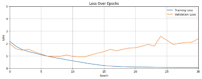
I built a function that takes the training and validation losses and the training and validation accuracies and plots them on graphs, allowing us to compare them and understand the model’s performance in a convenient, visual way. We’ll access these metric values through the history object we defined during model training.
def plot_training_history(history, metrics=("loss", "accuracy"), ylim_loss=(0, 5), ylim_acc=(0, 1)):
    """
    Plots the training and validation loss and accuracy.
    """
    for metric in metrics:
        plt.figure(figsize=(12, 4))

        train_metric = history.history[metric]
        valid_metric = history.history[f"val_{metric}"]

        plt.plot(train_metric, label=f'Training {metric.capitalize()}')
        plt.plot(valid_metric, label=f'Validation {metric.capitalize()}')

        plt.xlabel('Epoch')
        plt.ylabel(metric.capitalize())
        plt.title(f'{metric.capitalize()} Over Epochs')

        ylim = ylim_loss if metric == "loss" else ylim_acc
        plt.ylim(ylim)
        plt.xlim(0, len(train_metric) - 1)

        plt.legend()
        plt.grid(True)
        plt.show()
plot_training_history(history)
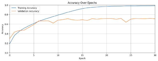
Before we make sense of the graphs, let’s revisit the difference between loss and accuracy:
- Loss: A scalar number measuring the gap between the model’s prediction and the actual class. In other words, the lower the loss, the better trained the model is.
- Accuracy: The ratio of correct predictions to the number of records in the dataset. For example, if its value is 0.95, the model identified the class correctly 95% of the time.
While the model performs well on the training data, it struggles to classify new images it has not seen before. How did I figure that out? A gap develops between training and validation after about 10 epochs. In other words, our model is overfitting, and we’ll need to make a compromise.
Adding Dropout #
There are several techniques for avoiding overfitting, one of which is adding dropout layers. What are they? Layers that randomly turn off some neurons during training. Turning off neurons limits the model’s ability to memorize the training data and allows it to represent general relationships.
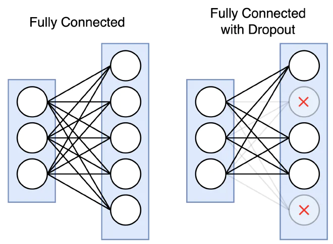
As you can see, the dropout layer will come after a max pooling layer and after an FC layer. For each dropout layer, we’ll define the percentage of neurons we want to randomly turn off during training.
Implementing the Model with a Dropout Layer #
def cnn_model_dropout(input_shape=(32, 32, 3)):
    model = Sequential()

    # ================================
    # Convolutional Blocks
    # ================================

    # ----- Conv Block 1: 32 Filters, MaxPool, Dropout -----
    model.add(Conv2D(filters=32, kernel_size=3, padding='same', activation='relu', input_shape=input_shape))
    model.add(Conv2D(filters=32, kernel_size=3, padding='same', activation='relu'))
    model.add(MaxPooling2D(pool_size=(2, 2)))
    model.add(Dropout(0.25))

    # ----- Conv Block 2: 64 Filters, MaxPool, Dropout -----
    model.add(Conv2D(filters=64, kernel_size=3, padding='same', activation='relu'))
    model.add(Conv2D(filters=64, kernel_size=3, padding='same', activation='relu'))
    model.add(MaxPooling2D(pool_size=(2, 2)))
    model.add(Dropout(0.25))

    # ----- Conv Block 3: 64 Filters, MaxPool, Dropout -----
    model.add(Conv2D(filters=64, kernel_size=3, padding='same', activation='relu'))
    model.add(Conv2D(filters=64, kernel_size=3, padding='same', activation='relu'))
    model.add(MaxPooling2D(pool_size=(2, 2)))
    model.add(Dropout(0.25))

    # ================================
    # Classifier
    # ================================

    model.add(Flatten())
    model.add(Dense(512, activation='relu'))
    model.add(Dropout(0.5))
    model.add(Dense(10, activation='softmax'))

    return model
We’ve defined a new model with dropout layers. In the Conv blocks, we configured 25% of the neurons to be turned off randomly, and in the FC layer, we configured 50%. The next step is to create, compile, and train it, exactly as we trained the model without dropout layers. Then we’ll display the results in graphs similar to the previous ones.
model_dropout = cnn_model_dropout()
model_dropout.summary()
Model: "sequential"
_________________________________________________________________
Layer (type)                Output Shape              Param #
=================================================================
conv2d (Conv2D)             (None, 32, 32, 32)        896

conv2d_1 (Conv2D)           (None, 32, 32, 32)        9248

max_pooling2d (MaxPooling2  (None, 16, 16, 32)        0
D)

dropout (Dropout)           (None, 16, 16, 32)        0

conv2d_2 (Conv2D)           (None, 16, 16, 64)        18496

conv2d_3 (Conv2D)           (None, 16, 16, 64)        36928

max_pooling2d_1 (MaxPoolin  (None, 8, 8, 64)          0
g2D)

dropout_1 (Dropout)         (None, 8, 8, 64)          0

conv2d_4 (Conv2D)           (None, 8, 8, 64)          36928

conv2d_5 (Conv2D)           (None, 8, 8, 64)          36928

max_pooling2d_2 (MaxPoolin  (None, 4, 4, 64)          0
g2D)

dropout_2 (Dropout)         (None, 4, 4, 64)          0

flatten (Flatten)           (None, 1024)              0

dense (Dense)               (None, 512)               524800

dropout_3 (Dropout)         (None, 512)               0

dense_1 (Dense)             (None, 10)                5130

=================================================================
Total params: 669354 (2.55 MB)
Trainable params: 669354 (2.55 MB)
Non-trainable params: 0 (0.00 Byte)
_________________________________________________________________
model_dropout.compile(
    optimizer=CompileConfig.OPTIMIZER,
    loss=CompileConfig.LOSS,
    metrics=CompileConfig.METRICS
)
# Train the Model (with Dropout)
history = model_dropout.fit(
    X_train,
    y_train,
    batch_size=TrainingConfig.BATCH_SIZE,
    epochs=TrainingConfig.EPOCHS,
    verbose=1,
    validation_split=TrainingConfig.SPLIT
)
Epoch 29/31
137/137 [==============================] - 45s 329ms/step - loss: 0.5194 - accuracy: 0.8156 - val_loss: 0.6442 - val_accuracy: 0.7786
Epoch 30/31
137/137 [==============================] - 45s 325ms/step - loss: 0.5028 - accuracy: 0.8214 - val_loss: 0.6675 - val_accuracy: 0.7780
Epoch 31/31
137/137 [==============================] - 45s 329ms/step - loss: 0.5005 - accuracy: 0.8235 - val_loss: 0.6622 - val_accuracy: 0.7771
plot_training_history(history)
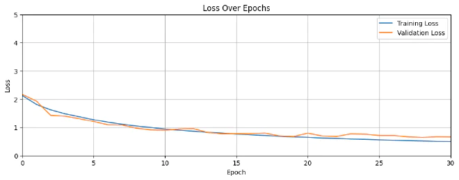
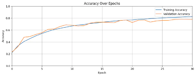
We can now see that we’ve managed to narrow the gap between training and validation, so adding dropout layers helped us prevent overfitting.
Saving and Loading the Model #
Training takes a few tens of minutes, and we don’t want to train the model every time we want to use it. That’s why it’s important to know how to save it after training and how to load it for future use.
Using the save() function, we can save the model in SavedModel format. After calling this function, a new folder will be created containing the model’s configuration, its weights, and statistical results about the model.
model_dropout.save('model_dropout')
INFO:tensorflow:Assets written to: model_dropout/assets
INFO:tensorflow:Assets written to: model_dropout/assets
We can then load it whenever we want using the load_model() function.
reloaded_model_dropout = models.load_model('model_dropout')
Model Performance #
There are several ways to measure the model’s performance (model evaluation). We can calculate accuracy on the test dataset, look at the model’s predictions visually, and create a confusion matrix.
Test Dataset #
We’ll load the images the model hasn’t seen from X_test y_test and use the evaluate function to compare the model’s predictions with the actual values.
test_loss, test_acc = reloaded_model_dropout.evaluate(X_test, y_test)
print(f"Test accuracy: {test_acc*100:.3f}")
313/313 [==============================] - 4s 12ms/step - loss: 0.6817 - accuracy: 0.7705
Test accuracy: 77.050
class_names = ['airplane', 'automobile', 'bird', 'cat', 'deer',
               'dog', 'frog', 'horse', 'ship', 'truck']
Sampling Images #
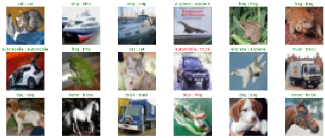
We’ll randomly select images from the test set and see what the model predicts compared with what is actually in each image.
import seaborn as sns
import matplotlib.pyplot as plt
import numpy as np
import tensorflow as tf

def evaluate_model(dataset, model, y_test, class_names):
    # Number of rows and columns for the plot grid
    num_rows, num_cols = 3, 6

    # Retrieve a batch of images from the dataset
    data_batch = dataset[0:num_rows*num_cols]

    # Get model predictions
    predictions = model.predict(data_batch)

    # Initialize variables
    num_matches = 0

    # Create plot
    plt.figure(figsize=(20, 8))

    for idx in range(num_rows * num_cols):
        ax = plt.subplot(num_rows, num_cols, idx + 1)
        plt.axis("off")
        plt.imshow(data_batch[idx])

        pred_idx = tf.argmax(predictions[idx]).numpy()
        truth_idx = np.argmax(y_test[idx])

        title = f"{class_names[truth_idx]} : {class_names[pred_idx]}"
        title_color = 'g' if pred_idx == truth_idx else 'r'

        plt.title(title, fontsize=13, color=title_color)

        num_matches += (pred_idx == truth_idx)

    acc = num_matches / (num_rows * num_cols)
    print(f"Prediction accuracy: {acc:.2f}")

    plt.show()

evaluate_model(X_test, reloaded_model_dropout, y_test, class_names)
1/1 [==============================] - 0s 24ms/step
Prediction accuracy: 0.89
Confusion Matrix #
We use a confusion matrix when we want to compare the actual and predicted values of labels. This matrix lets us assess the model’s correctness at the class level. A class-level comparison can show us whether the model confuses certain classes, allowing us to refine it accordingly.
# Generate predictions for the test dataset.
predictions = reloaded_model_dropout.predict(X_test)

# For each sample image in the test dataset, select the class label with the highest probability.
predicted_labels = [np.argmax(i) for i in predictions]
313/313 [==============================] - 4s 12ms/step
# Convert one-hot encoded labels to integers.
y_test_integer_labels = tf.argmax(y_test, axis=1)

# Generate a confusion matrix for the test dataset.
cm = tf.math.confusion_matrix(labels=y_test_integer_labels, predictions=predicted_labels)

# Plot the confusion matrix as a heatmap.
plt.figure(figsize=[14, 7])
sns.heatmap(cm, annot=True, fmt='d', annot_kws={"size": 12})
plt.title('Confusion Matrix')
plt.xlabel('Predicted')
plt.ylabel('Truth')
plt.show()
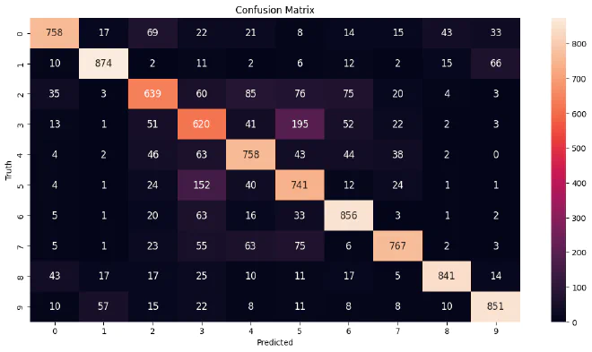
We can see that the model confuses dogs with cats, and trucks with cars. This confusion makes sense given the very low resolution of the images.
Explainable AI #
In my opinion, being able to explain a model’s results is just as important as its correctness. That’s why I decided to devote another section of this article to Explainable AI. There’s a perception that AI models are black boxes that cannot be explained, and I took on the challenge of explaining a CNN model.
The Model’s Layers #
As we’ve learned, a CNN model has Conv layers with different sizes, depths, and filters. I thought it would be interesting to see how the image changes as it passes through the model.
- We’ll store a representation of the model’s Conv layers (by index) in the
conv_layer_indicesarray. - We’ll randomly select 5 images from
X_test. - We’ll display the images.
- For each image:
- We’ll take the last filter in the last layer of each Conv block.
- We’ll perform a Conv operation on the image, so that the second block receives the result of the second, and so on.
- We’ll display the filter and the multiplication result.
conv_layer_indices = [0, 1, 4, 5, 8, 9]

# Randomly select 5 images from X_test
random_indices = np.random.choice(X_test.shape[0], size=5, replace=False)
selected_images = X_test[random_indices]

# Create a figure to display the original images once
plt.figure(figsize=(20, 4))

# Add an empty subplot for alignment
plt.subplot(1, 6, 1)
plt.axis('off')

# Display original images
for j in range(5):
    plt.subplot(1, 6, j + 2)
    plt.imshow(selected_images[j].astype('uint8'))  # Assuming the images are normalized
    plt.axis('off')
plt.show()

# Loop through the convolutional layer indices
for idx in conv_layer_indices:
    filters, _ = model.layers[idx].get_weights()

    # Get the last kernel from the layer
    last_kernel = filters[:, :, :, -1]

    # Create a truncated model that ends at this layer
    truncated_model = Model(inputs=model.inputs, outputs=model.layers[idx].output)

    # Generate feature maps for the selected images
    feature_maps = truncated_model.predict(selected_images, verbose=0)  # Setting verbose to 0

    # Create a figure to hold the last kernel and the affected images
    plt.figure(figsize=(20, 4))

    # First subplot: Last kernel
    plt.subplot(1, 6, 1)
    plt.imshow(last_kernel[:, :, 0], cmap='gray')  # Assuming single channel (grayscale)
    plt.axis('off')

    # Next subplots: Affected images
    for j in range(5):
        affected_image = feature_maps[j, :, :, -1]
        plt.subplot(1, 6, j + 2)
        plt.imshow(affected_image, cmap='gray')
        plt.axis('off')
    plt.show()
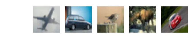






Now you can get a sense of which regions of the image the model is looking at, which patterns it has extracted, and how the image is processed throughout the model.
Through the Model’s Eyes #
Now that we’ve seen how the model processes an image, the natural next step is to see which regions it focuses on, what it predicts is in the image, and what is actually there.
- Selecting images
- We’ll randomly select 50 images from
X_test. - We’ll retrieve the name of the object in each image.
- We’ll randomly select 50 images from
- Prediction: For each image, we’ll examine the model’s prediction using the
predict()function. - Submodels: We’ll split the CNN into parts according to
conv_layer_indices(the positions of the Conv blocks in the model). - Visualization: We’ll define
figandaxes, which we’ll use to display the images. - Calculating a heatmap: For each image:
- We’ll display its original version.
- We’ll calculate the result of multiplying the image through the separated layers of the model.
- We’ll display the multiplication result and the model’s prediction.
- We’ll make display adjustments.
# Randomly select 50 images from X_test
num_images = 50
random_indices = np.random.choice(X_test.shape[0], num_images, replace=False)
selected_images = X_test[random_indices]
selected_labels = [class_names[label[0]] for label in y_test[random_indices]]

# Get the model's predictions for the selected images
predictions = model.predict(selected_images)
selected_labels = [class_names[label[0]] for label in y_test[random_indices]]

# Create sub-models to get the output of each selected conv layer
layer_outputs = [model.layers[i].output for i in conv_layer_indices]
sub_models = [Model(inputs=model.inputs, outputs=output) for output in layer_outputs]

# Initialize a figure for plotting
fig, axes = plt.subplots(num_images // 2, 4, figsize=(20, (num_images // 2) * 4))

for i in range(num_images // 2):
    for j in range(2):
        idx = i * 2 + j
        img = selected_images[idx]
        label = selected_labels[idx]
        pred_label = predicted_labels[idx]

        # Display original image
        axes[i, j * 2].imshow(img)
        axes[i, j * 2].set_title(label)
        axes[i, j * 2].axis('off')

        # Compute and plot heatmaps
        heatmaps = []
        for sub_model in sub_models:
            conv_output = sub_model.predict(img[np.newaxis, ...], verbose=0)
            resized_heatmap = resize(conv_output[0, :, :, -1], (img.shape[0], img.shape[1]))
            heatmaps.append(resized_heatmap)

        # Sum the resized heatmaps
        summed_heatmap = np.sum(heatmaps, axis=0)

        # Normalize the summed heatmap
        summed_heatmap = (summed_heatmap - np.min(summed_heatmap)) / (np.max(summed_heatmap) - np.min(summed_heatmap))

        # Display the overlay
        axes[i, j * 2 + 1].imshow(img, alpha=1.0)
        axes[i, j * 2 + 1].imshow(summed_heatmap, cmap='jet', alpha=0.6)
        axes[i, j * 2 + 1].set_title(pred_label)  # Set the title to the model's prediction
        axes[i, j * 2 + 1].axis('off')

plt.tight_layout()
plt.show()
I didn’t choose to show 50 images for no reason. We can learn a great deal about the model from this visualization. For example, it recognizes a cat by its outline, a horse by its legs, a car by its outline, and other interesting features. We can also see why the model confuses labels and make corresponding changes to the model or the dataset. Even though the images are very small, we can extract interesting insights from the model we’ve built.

Closing Thoughts #
In this article, we learned how to use Tensorflow to build and train a basic CNN model. We learned about overfitting and about adding dropout layers to reduce it. We learned techniques for evaluating the model’s results, and finally, we visualized how the model sees.